1
Shape Maker manual.
Contents
Shape Maker manual
1
Installation and first run
4
Software installation
4
Start the program
4
Overview of the program interface
6
The outlook of the work window
6
Main Menu
8
Toolbars
9
Working window of the program
10
The Model blocks tree
10
The Properties window of the item
11
Commands and Messages History window
11
The coordinates input window
11
The status bar
12
Concepts
15
The coordinate system of the object
15
Units
15
The coordinate grids
16
Work plane
19
The sections plane
22
Model projection
23
Controls the visual representation of the model
23
The presentation of model elements
24
Points
24
Lines
24
Surfaces
24
Visualize the model's working volume
26
The visibility of objects in the block tree
28
Select items to edit
31
Select a group of items
31
Specifies the outline of a lines set
31
The current block and color
32
Cursor modes
32
Moves the cursor in a horizontal or vertical direction
33
Moves the cursor in the specified direction
33
Move the cursor in the orthogonal direction to the given angle
34
Scaled move the cursor in the specified direction
34
Change the coordinates of the mouse point
35
2
Mathematical model
36
Point
36
Line
36
Surface
37
Driver
37
Links
38
The element names
38
The topological dependency of the elements
38
The topological relationship of the elements
38
The object snap
40
Snaps to a point by two coordinates
41
Snaps to a point by three coordinates
41
Topological snap to point
41
Snaps to a line by two coordinates
41
Snaps to a line by three coordinates
41
Topological snap To line
41
Snaps to a mesh node
42
Snaps to the point of intersection of a line with one of the grid lines
42
Snaps to a line with the exact job of one of the coordinates
42
Working with lines
43
Specifies the spatial lines
43
Specifies the surface lines
45
Changes the shape of the spatial lines
49
To change the position of line endpoints
49
Edits the shape of the curve
49
Changes the number of control polygon points
50
Specifies the tangents at the end points of the curve
52
Fillet curves
55
Straightening lines
57
Edits the Polygon Control Point group
59
Modes of changing the shape of the curve when the position of its end point changes
62
Smoothing Form Curve
66
Changes the shape of the lines that lie on the surface
71
Working with surfaces
73
The surfaces definition
73
Controls the number of surface control points
75
Surface visualization
77
Line of an equal surface parameter
78
Surface intersection lines with a set of orthogonal planes
78
Shaded surfaces
79
Edit surfaces
81
Changes the position of corner points on the surface
82
Changes the shape of a surface boundary line
85
3
Changes the position of the control polyhedron points on the surface
86
Smooth connection of surface patches
90
Straightening a number of surface control points
92
Smooth connection of surfaces with orthogonal planes
94
Surface smoothing
96
Visualization of the curvature Chart of cross-sections and inflection lines
98
First project
104
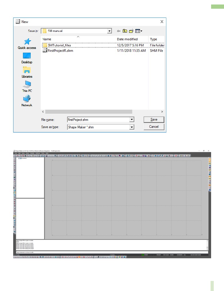
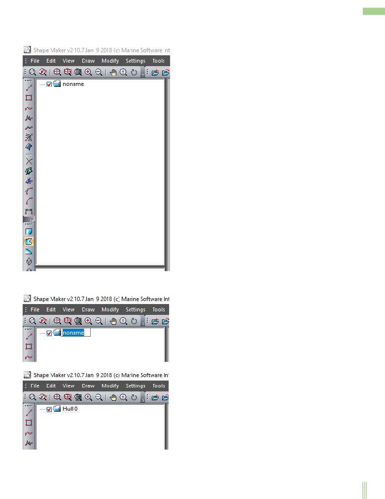
Create a new project
104
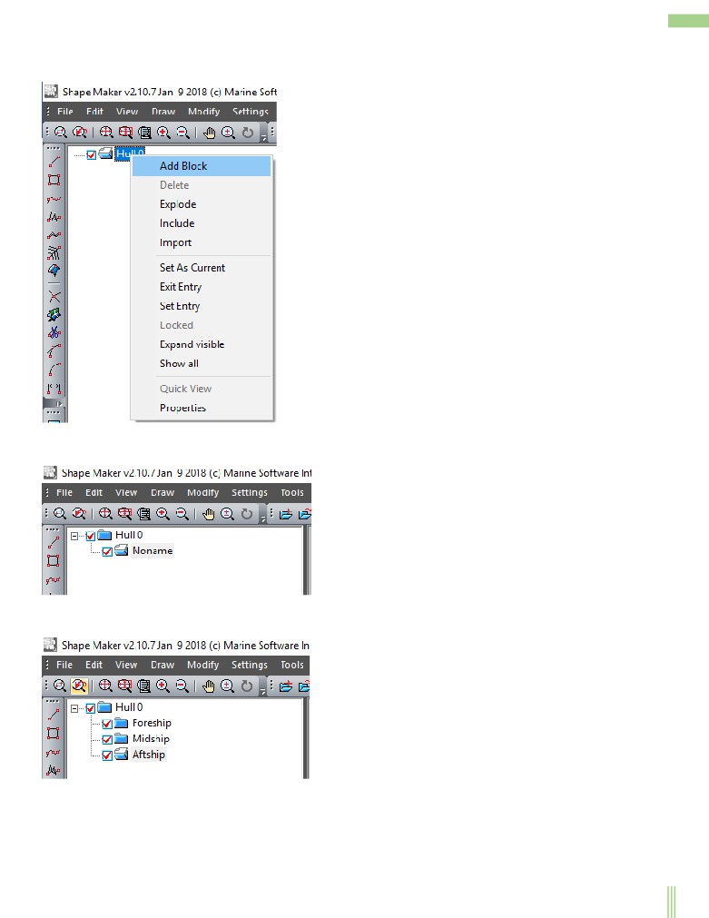
Создание структуры блоков проекта
106
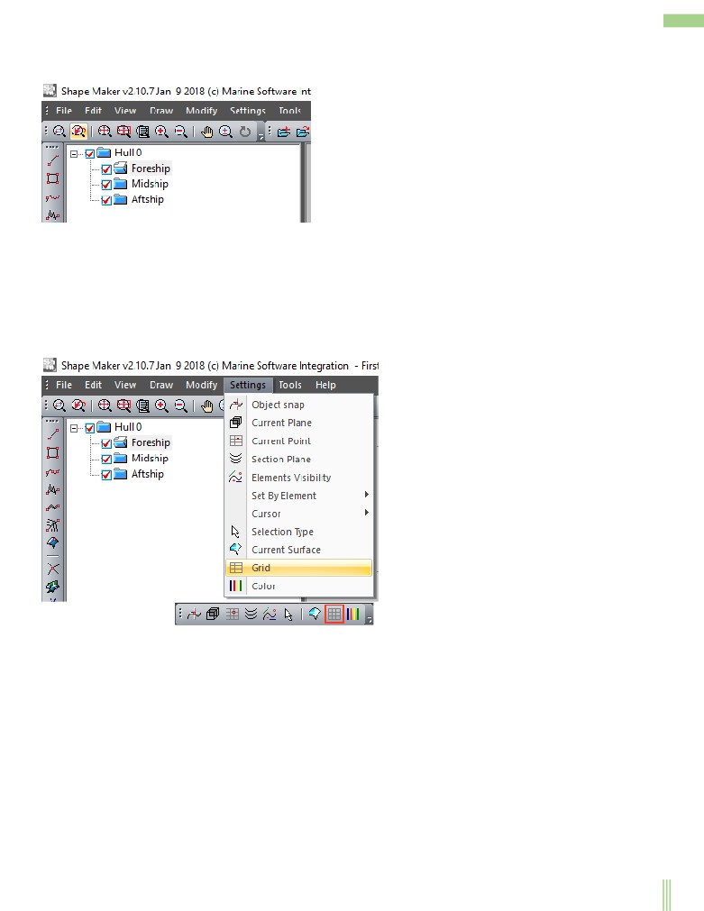
Specifies the grid
108
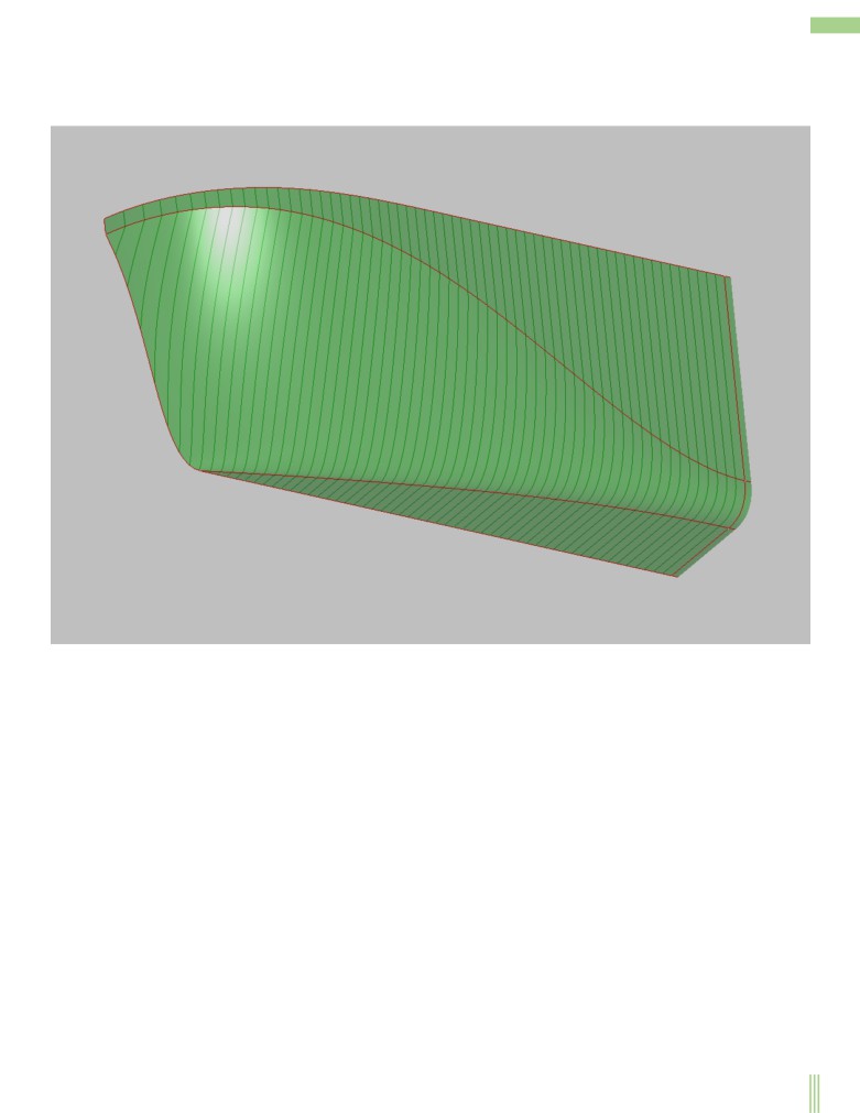
Modeling the fore ship
113
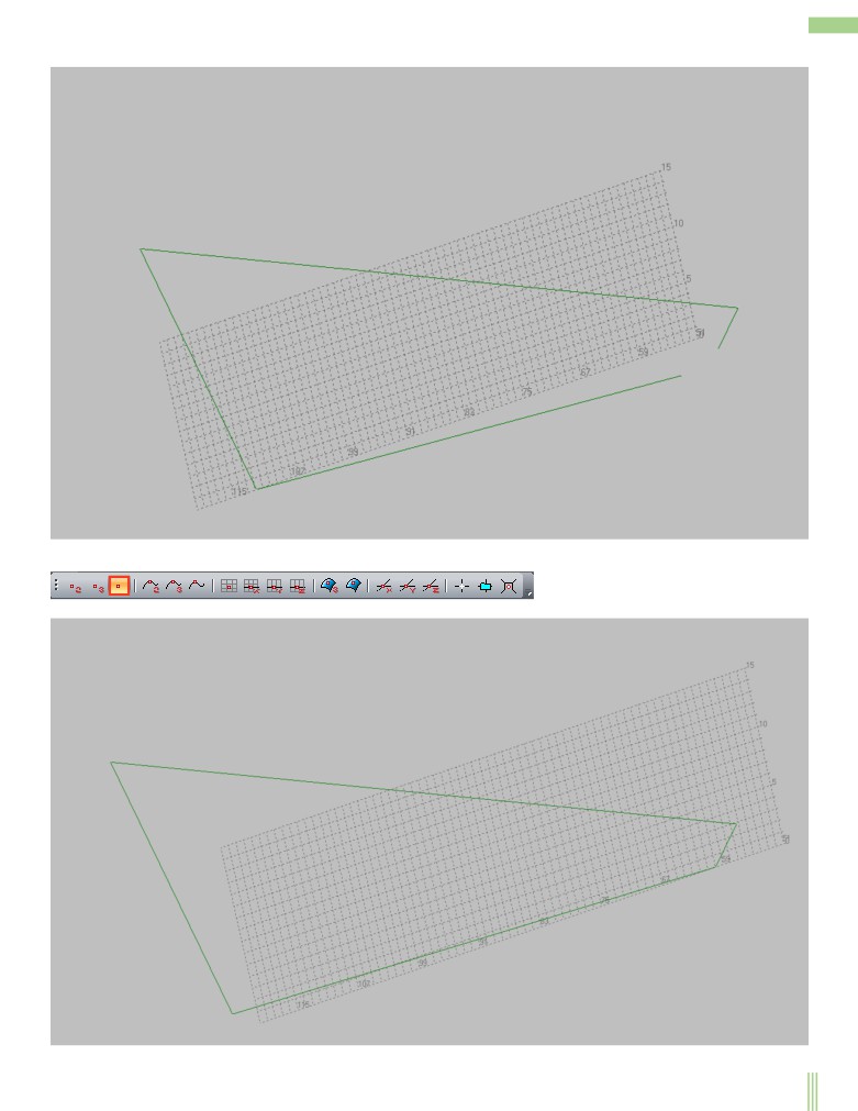
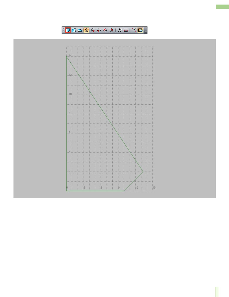
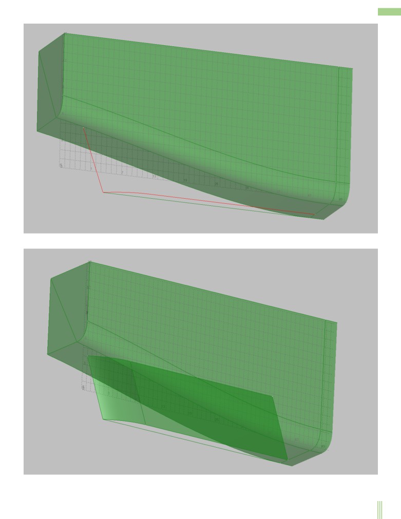
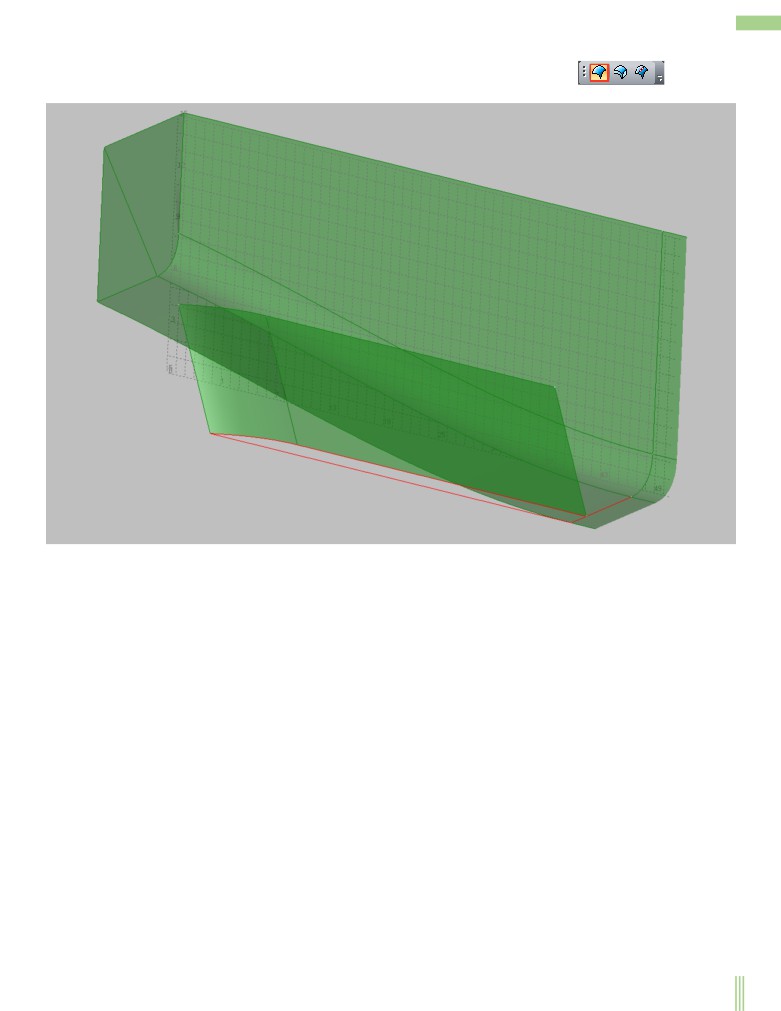
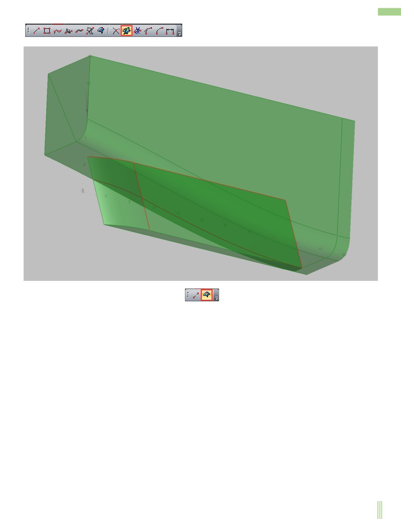
Specifies the boundary lines of the curved surface area
114
Sets and edits a surface patch
121
Specifies the surfaces of the flat board and the flat bottom of the fore ship
134
Modeling of parallel midbody surface
138
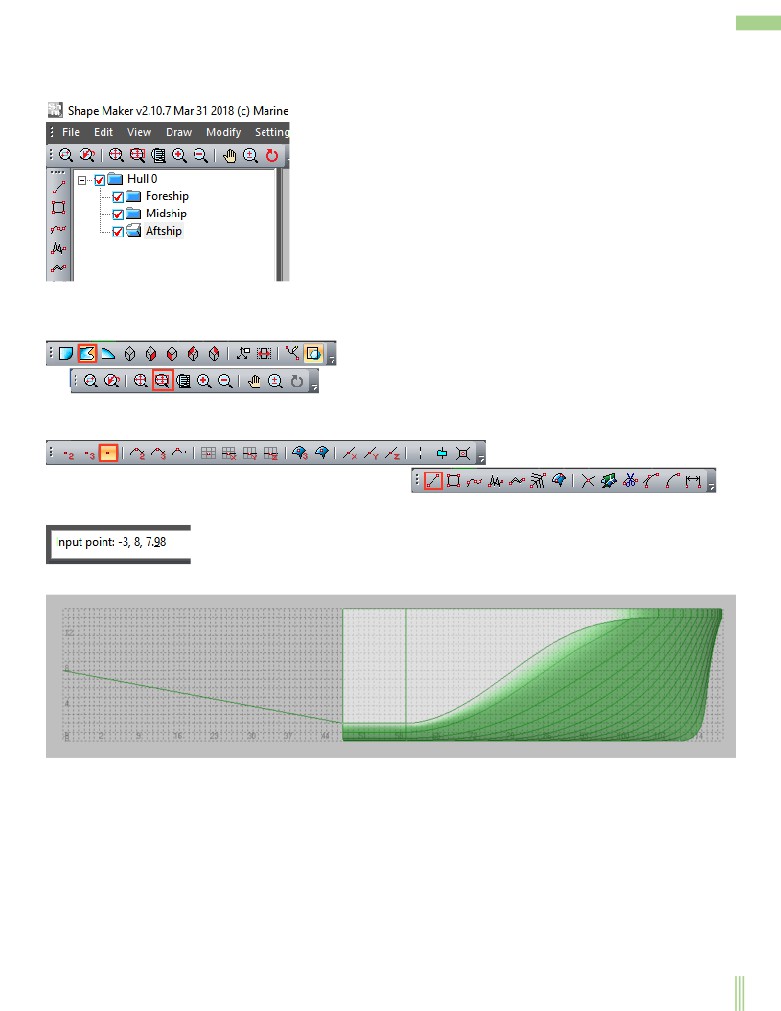
Simulation of aft ship
142
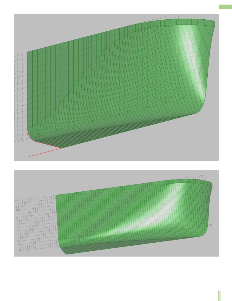
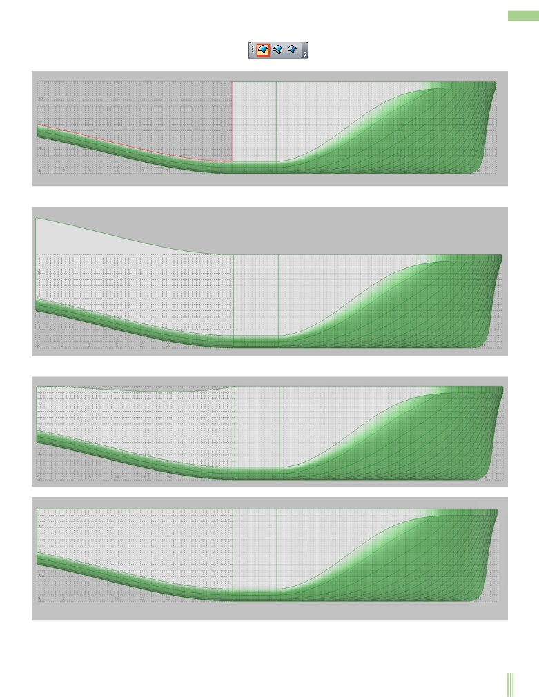
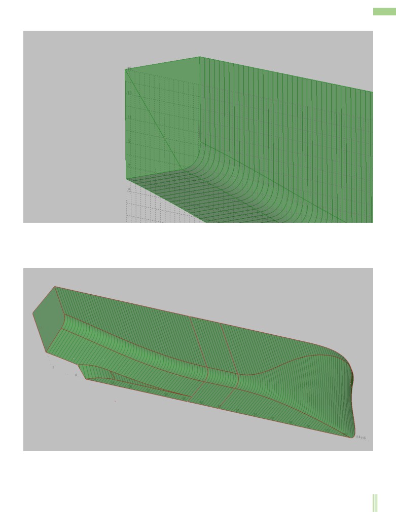
Modeling of the main surface of the aft ship
142
Modeling of transom
145
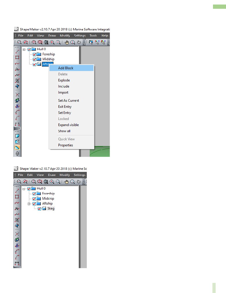
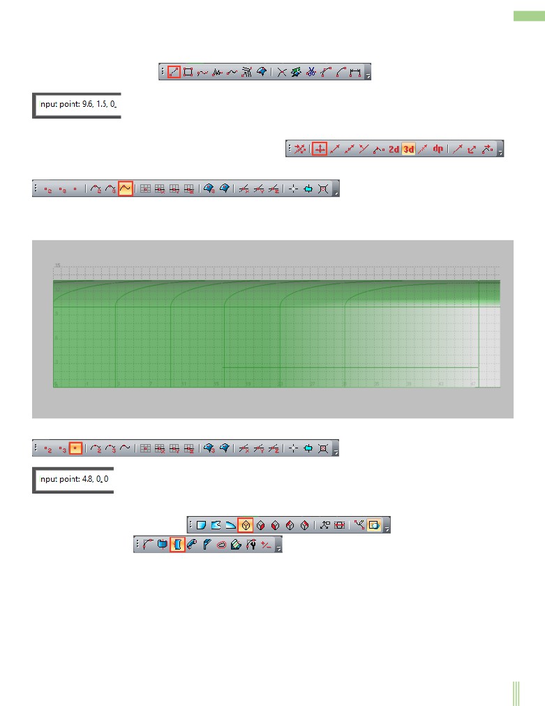
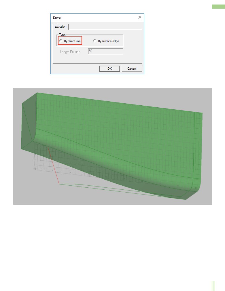
Modelling of the surface of fodder skeg
149
4
Installation and first run.
Software installation.
Installation of the program is quite simple and does not require any special skills. Just run the installation file and follow the
instructions. There are no special requirements for installing the program. The installation files and the program itself take up very
little disk space. The only condition for running the program is that the computer has a graphics card that supports OpenGL. Virtually
any computer currently supports OpenGL graphics. Almost any computer with a processor of any performance will take less than a
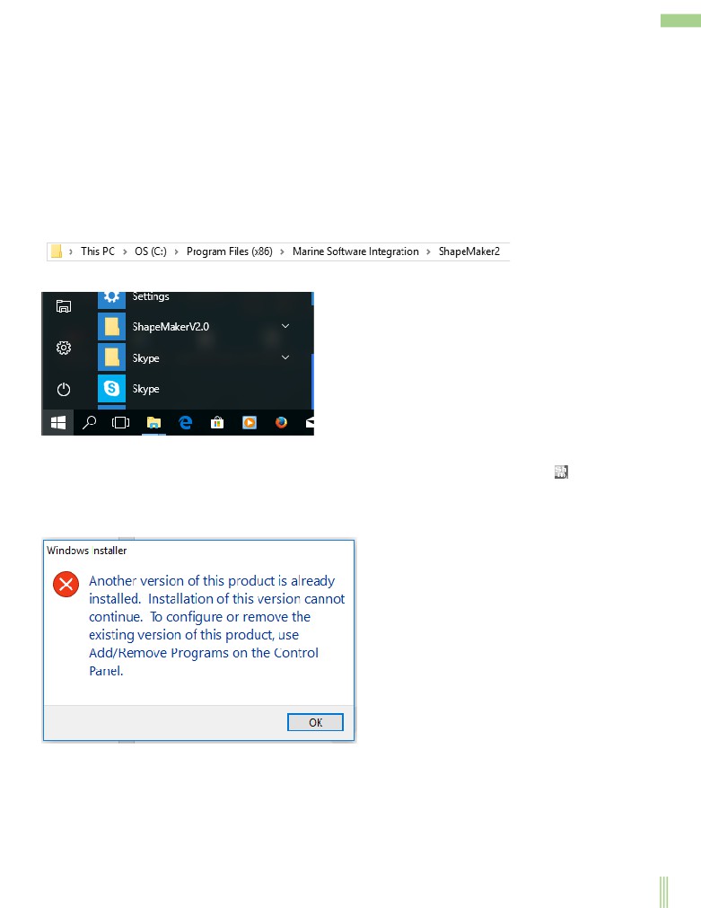
minute to install. As a result of installation of the program on the system disk in the directory "program Files (86)" The catalogue
"Marine Software Integration" and subdirectory "Shapemaker2" will be created. All files related to the program will be in this
subdirectory.
A subdirectory is added to the list of installed Windows programs “ShapeMakerV2.0”.
The standard file of the program project has the extension "SHM". From this moment all files with extension "SHM" will be opened
by the program. After installation of the program all files with extension "SHM" will have a characteristic icon
A license must be connected to start the program.
If the program has already been installed on your computer, the following message appears:
Always before you install a new version of the program, you must first uninstall the old version.
Start the program.
The program can be launched in three different ways:
- from the catalog menu of the installed Windows programs,
- directly from the directory where the executable file of the program-Shapemaker.exe is located,
- by double-clicking on the project file with Extension "SHM".
5
License.
Currently, the program supports two types of licenses:
- Network license. This license is installed on the license server located on the local network. To connect the program to such license
you need to enter the server name or its IP address and port. You can find this information from your system administrator. Upon
request, the license server checks for free licenses and allows the program to run.
- Local license. The local license is contained in the license. txt file which must be in the same directory as the executable file of the
program.
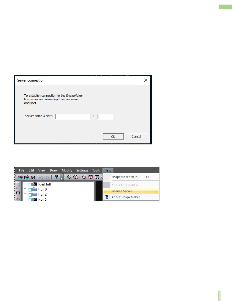
When running, the program tries to find the local license file, if this file is not found, the program tries to connect to the license server.
If this fails, a menu appears that requires you to enter the correct IP address and port of the license server:
If a connection to the license server is established, but no licenses are available, a message is issued and the program stops working.
If you need to change the server name or port in the process, you can call the dialog and the following menu:
The installation process of the license server is not described in this manual and is information for the system administrator.
6
Overview of the program interface.
This section shows the main details of the program interface.
The outlook of the work window.
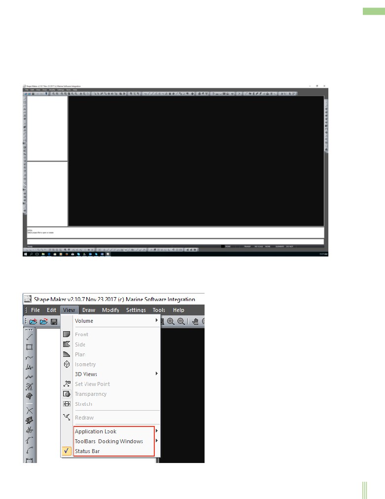
When you first start the program after a successful installation, you will see a window like this:
This shows the initial location of the default interface elements. During the work, the user can configure the location of the program
and toolbar windows at their own discretion. Note that most of the commands are not active at this time because the project is not
loaded. To change the position of the interface elements, the user can use the standard Windows tools. The program also provides the
following commands:
That will change the appearance of the application location visualization of toolbars and bar status.
7
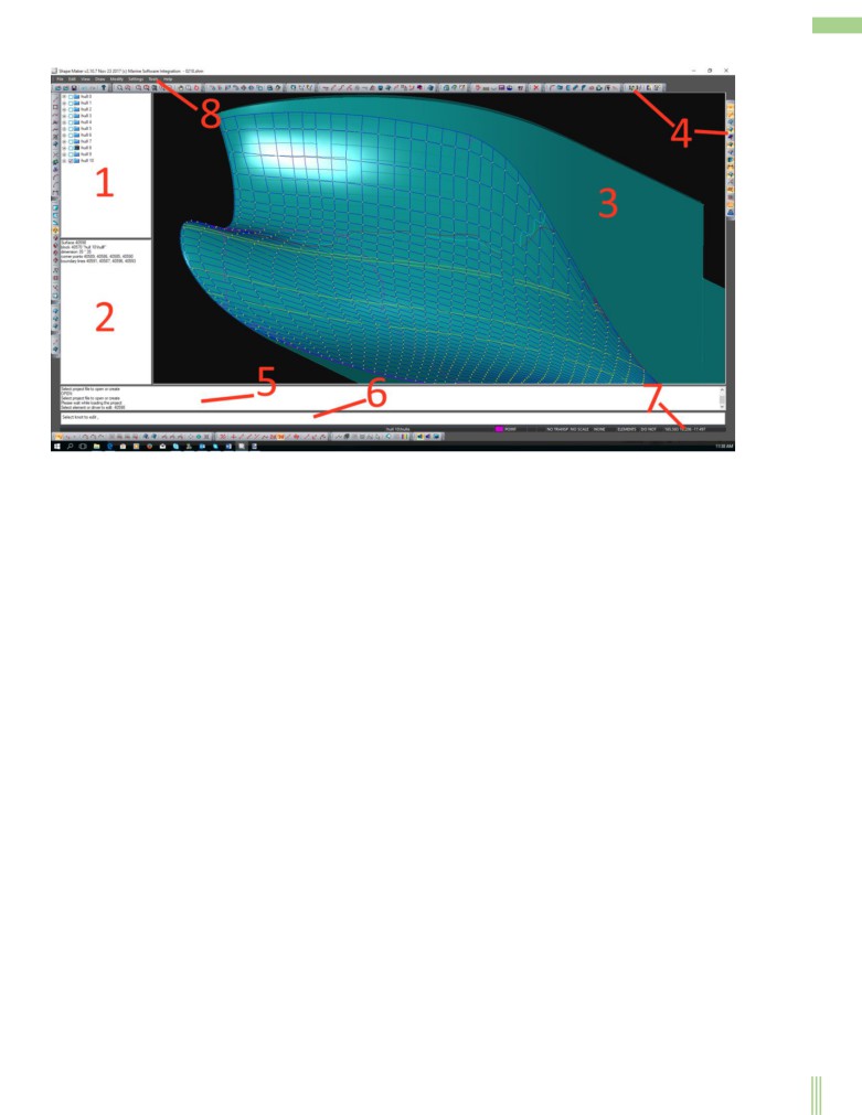
The following image shows the location of the interface elements:
1-The Project block tree window,
2- the Properties window of the item selected for editing,
3- the program window,
4- the toolbars,
5- the command and Message History window,
6- the coordinate input window,
7- the status bar,
8- the main menu.
In the process of working with the program, you can also see context menu and dialog boxes.
8
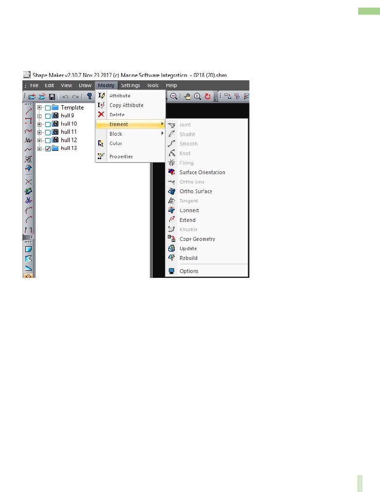
Main Menu.
The menu contains the full set of commands available at the moment. Depending on the mode of the program, some menu items may
not be available. The command icon that is currently active is highlighted more vividly. Some menu items, divided by semantic
principle, may contain subparagraphs.
9
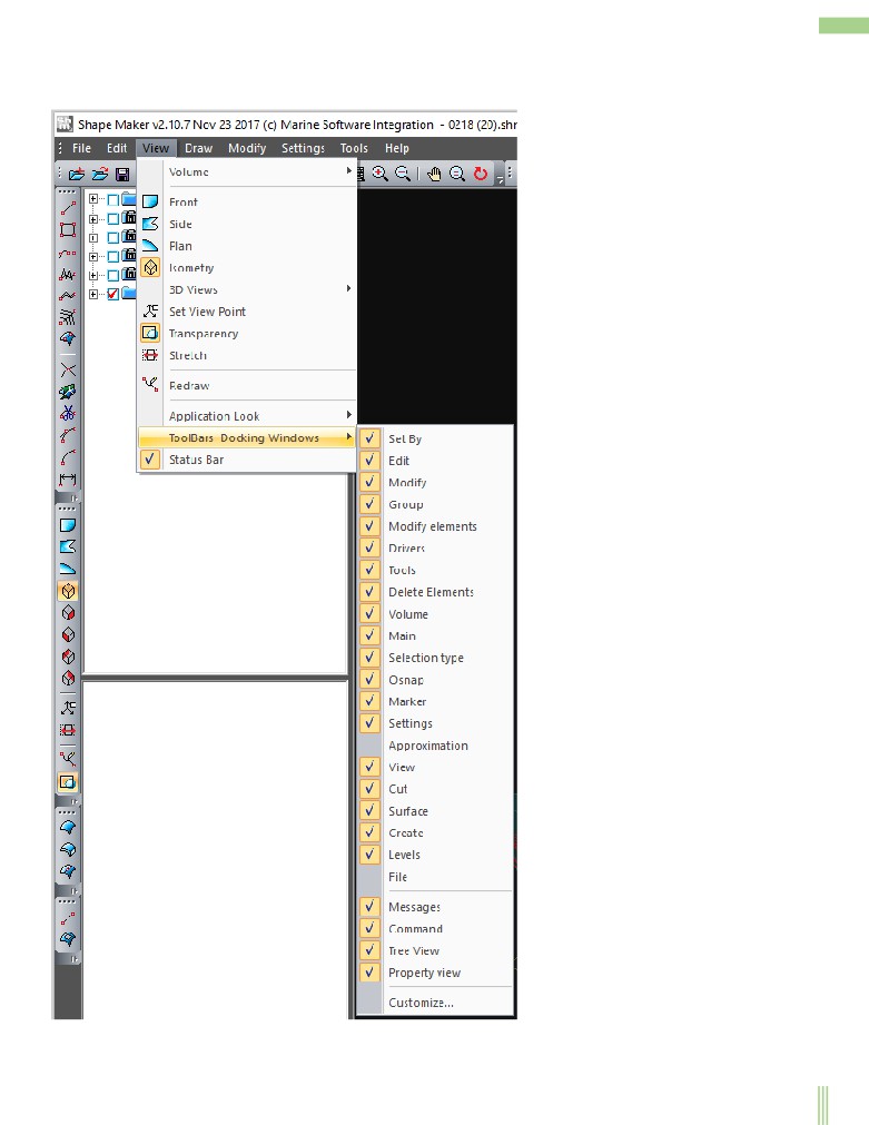
Toolbars.
The full list of toolbars can be seen here:
All toolbars are divided into thematic groups and are the most convenient way to use commands.
10
Working window of the program.
The program's working window is used for input and output of graphic information.
The Working window displays the image and generates a mathematical model (entering and editing lines and surfaces).
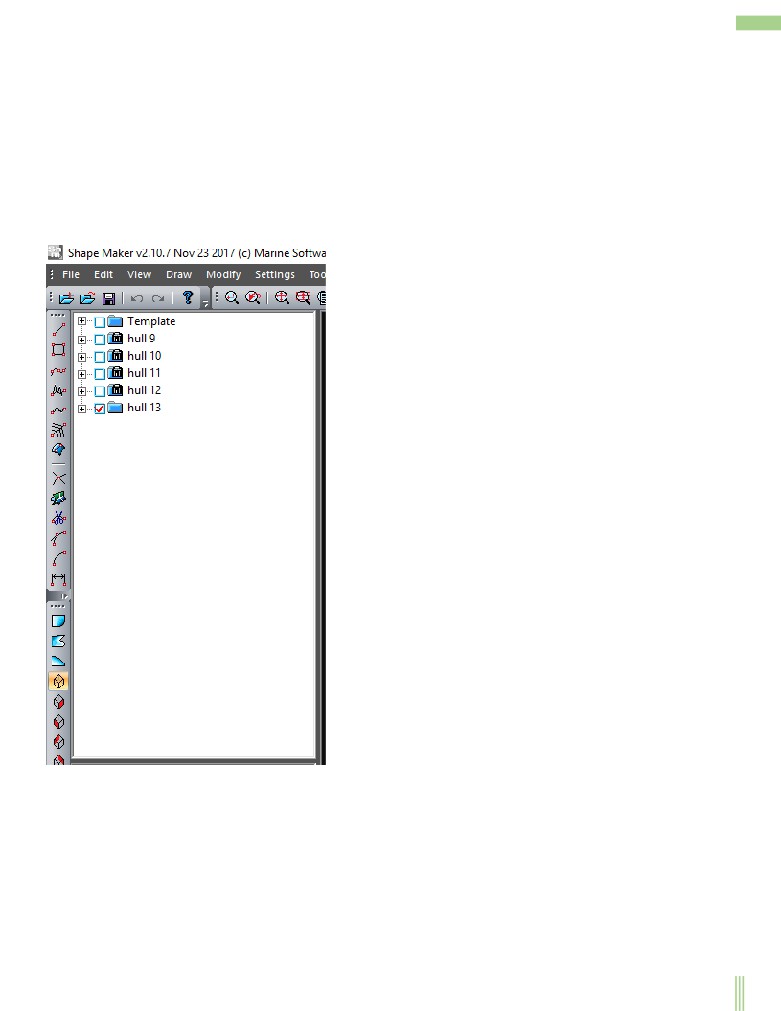
The Model blocks tree.
The Model blocks tree allows you to add or remove blocks, enable, disable, make the current block of the project and do other
necessary actions with the blocks of the tree. All changes in the block tree will be automatically reflected in the model that is in the
work window. So, if one block is turned off in the blocks three window, all elements that are included in this block will no longer be
displayed in the program's work window.
11
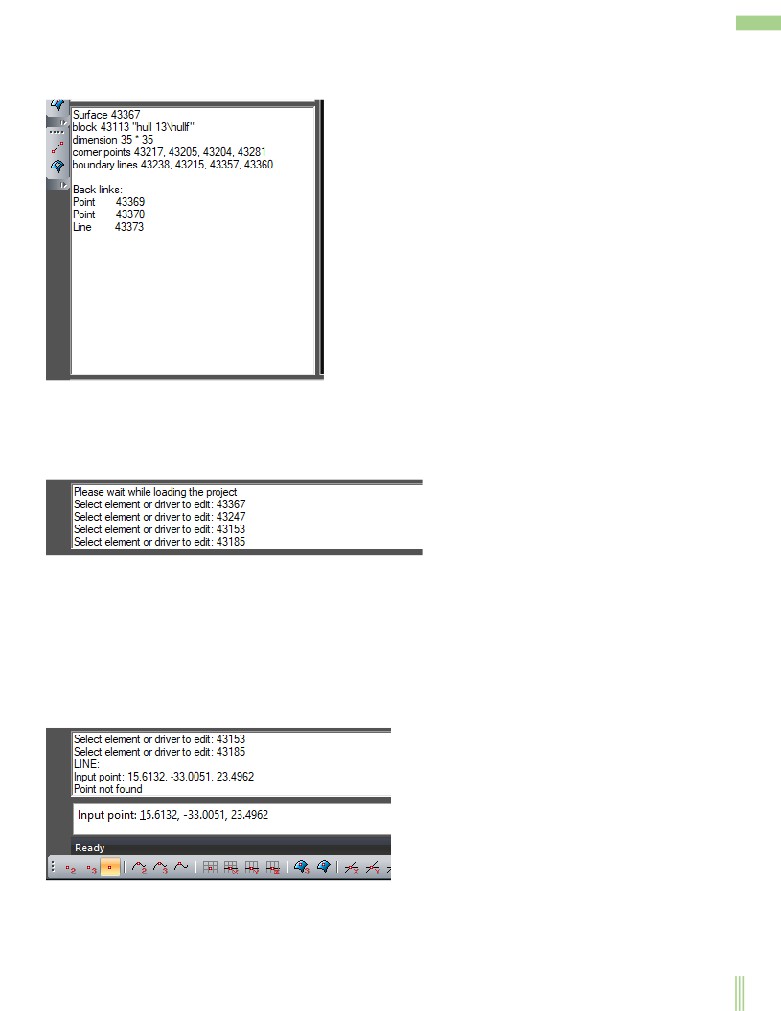
The Properties window of the item.
Use this window to display the properties of the current item selected for editing.
Commands and Messages History window.
All executed commands, error messages and other messages are displayed in the Command History window. This window allows you
to view all the commands for the work session.
The coordinates input window.
A special input window is used if you want to specify the exact point’s coordinates.
The user can enter the coordinates of the points using the mouse cursor, and the input window displays the coordinates of the previous
point. If during work, there is a necessity of exact definition of coordinates, it is enough to click in a field of an input window (or to
press the arrow button left/right on keyboard) and to edit coordinates of the previous point. If you want to enter new coordinates of a
point, simply press the numeric key on the keyboard and the system will switch to the coordinate input mode. This will clear the input
window field from the coordinates of the previous point.
12
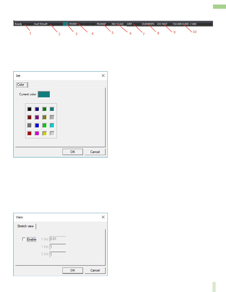
The status bar.
The status bar contains several fields:
1 - A field indicating the status of the active window if the cursor is in the window. If you hover over one of the toolbar buttons, this
field will show the ToolTip for that button.
2 - A field indicating the current project block.
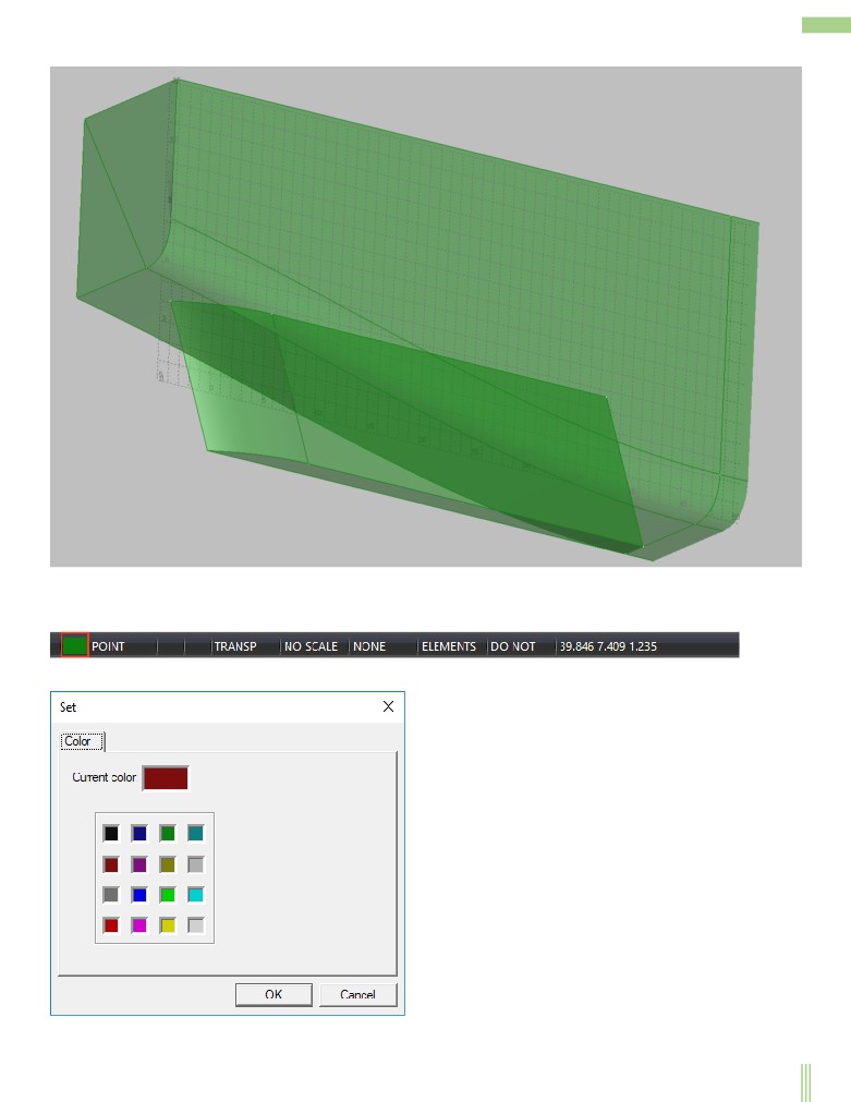
3 - Field of the current color of input elements. If you click this box, a dialog box will appear allowing you to change the color of the
item you are defining.
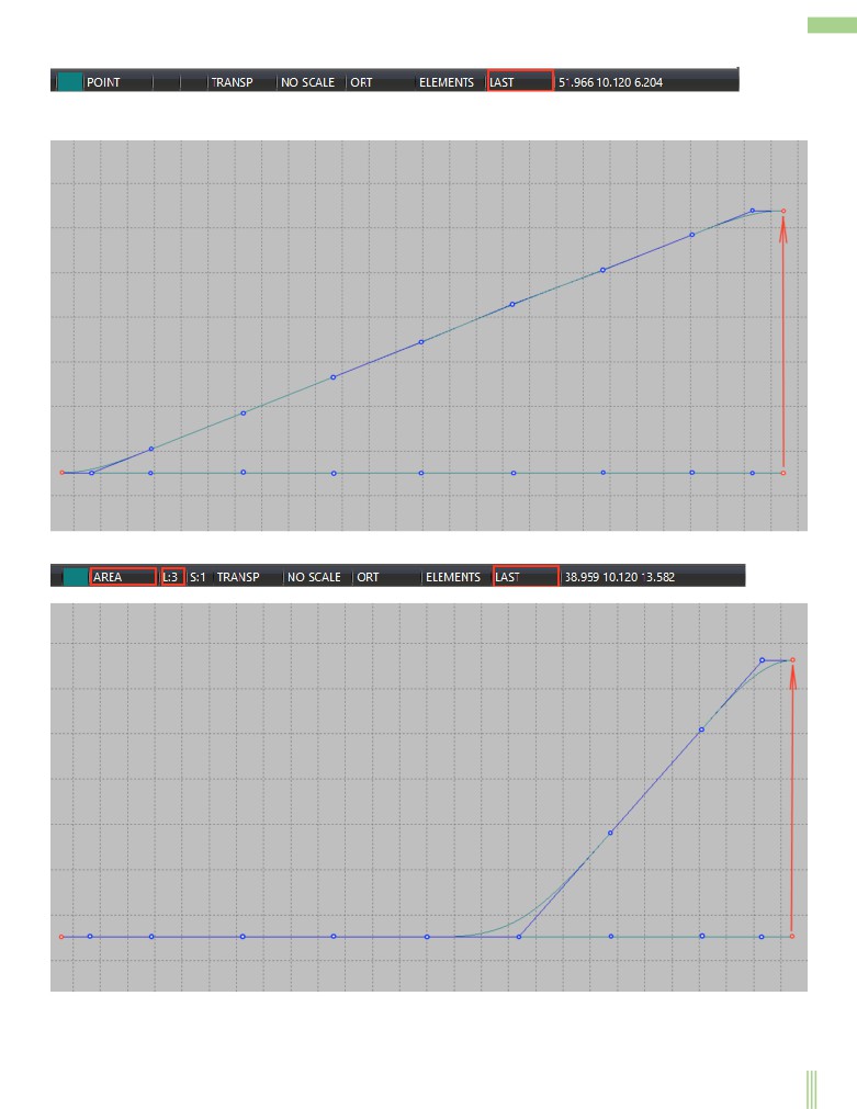
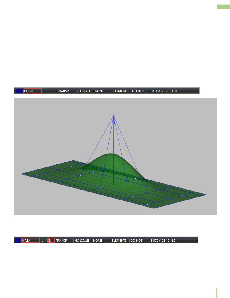
4-field of line and surface editing mode setting. In POINT mode, you always edit only one control point on a line or surface. In area
mode, you edit a line or surface control point’s group. In this mode, the following two fields become active: These fields define the
scope of the control point area change. You can zoom in and out of the change area by clicking the left or right mouse button,
respectively.
5 — This field is responsible for the transparency of the surface visualization. In TRANSP mode, the surface is rendered as semi-
transparent. In the NO TRANSP mode, the surface is not transparent. You can switch the transparency mode by clicking the mouse in
this field.
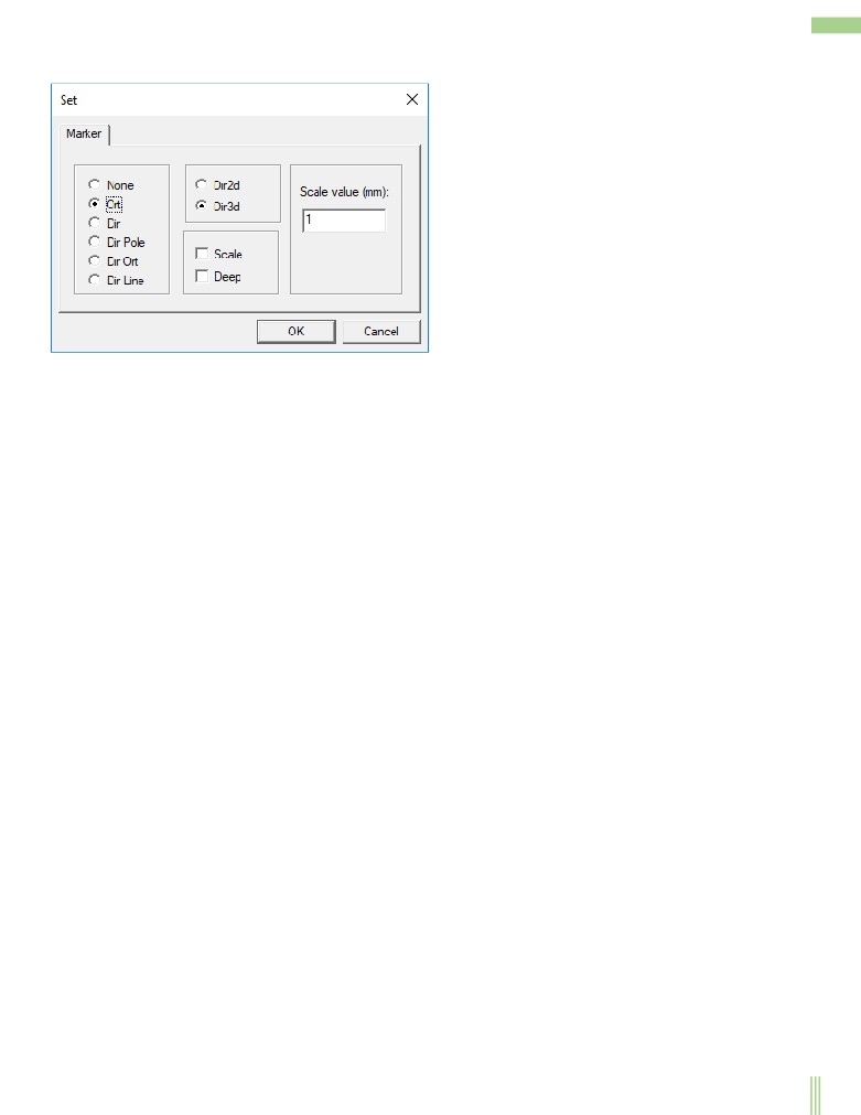
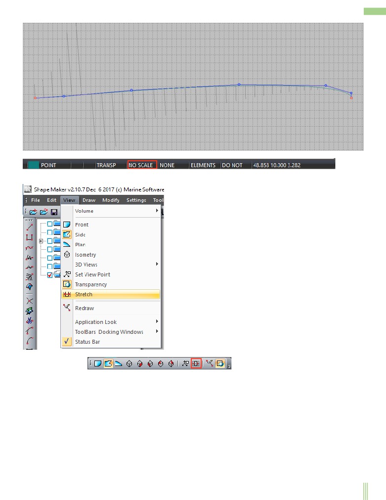
6 - This field is responsible for scaling the image on the screen. In mode NO SCALE displays the real image of the object, in the scale
mode displays a compressed image of the object according to the compression ratios of the coordinate axes. Switching modes is done
by mouse click in this field. If you do not specify compression ratios when you select a mode, the following menu is displayed:
13
7-This field shows the mode of the cursor. If you click the left mouse button in this field, a menu of the cursor mode will appear.
8-This field shows the current selection mode of the items. There are three options:
- ELEMENTS- element by element selection,
- BLOCK - Select the entire block when you specify one of the objects included in this block
-TREE - Select a block directly from the tree block window.
These modes are switched by pressing the left mouse button of this field.
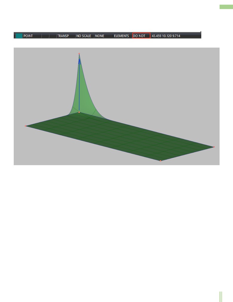
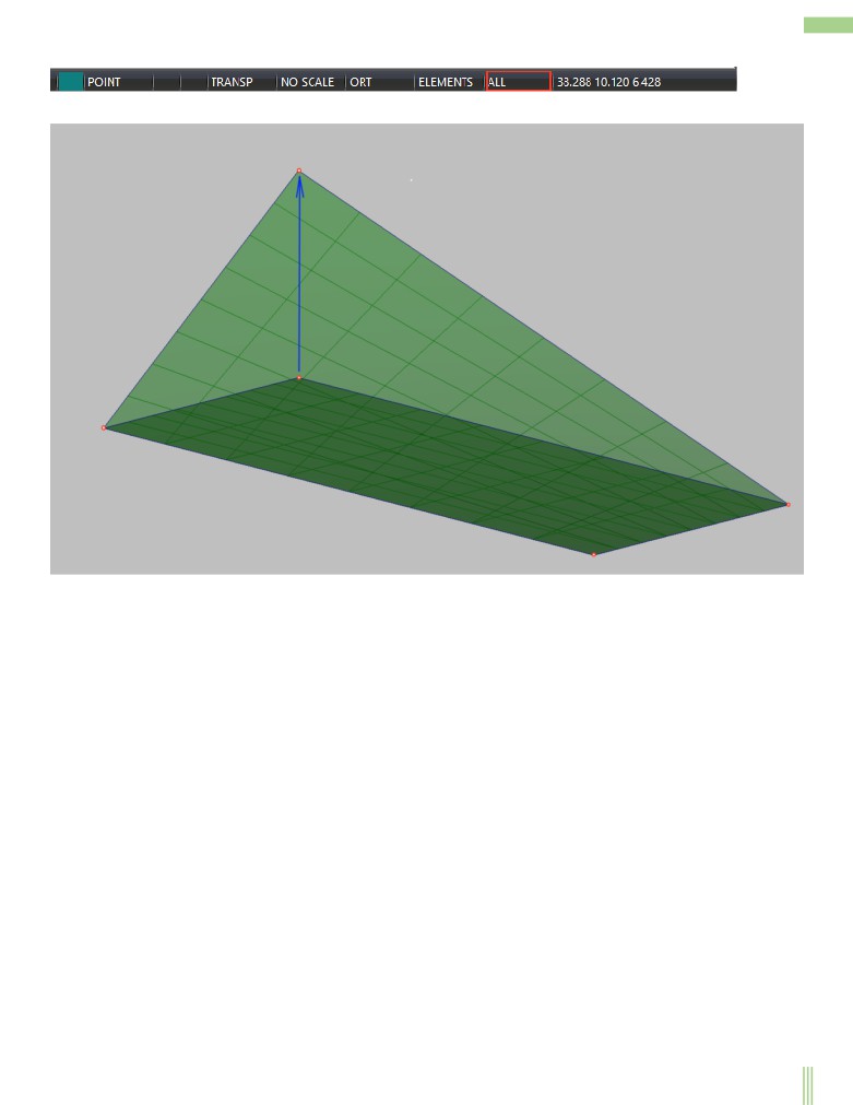
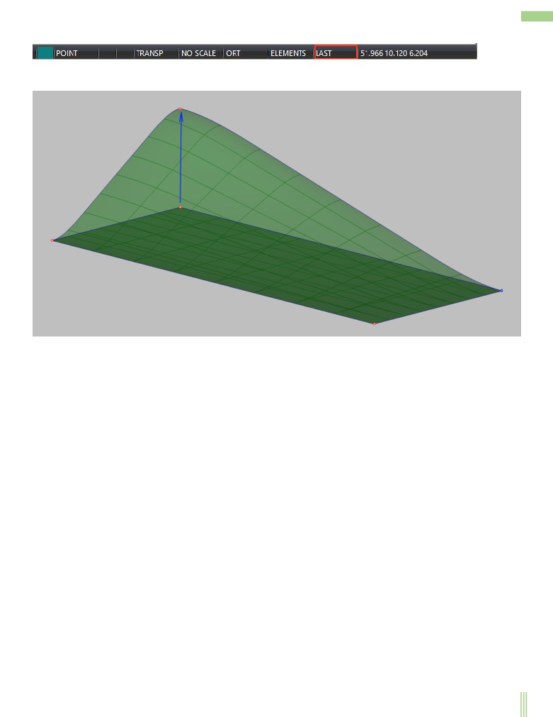
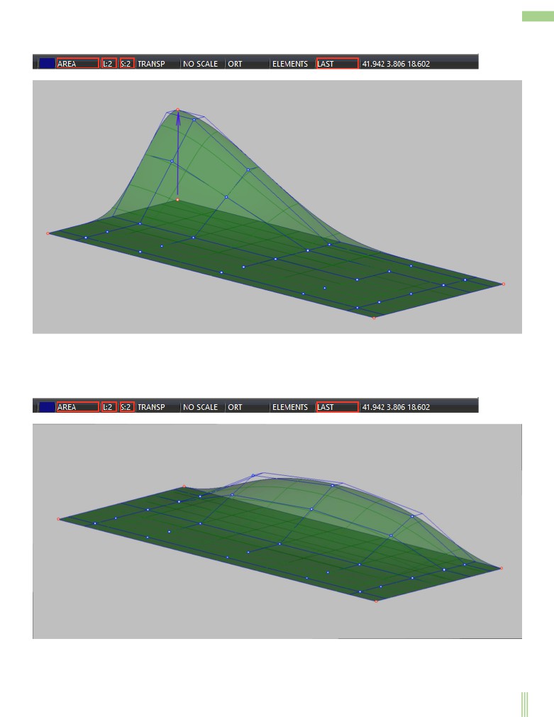
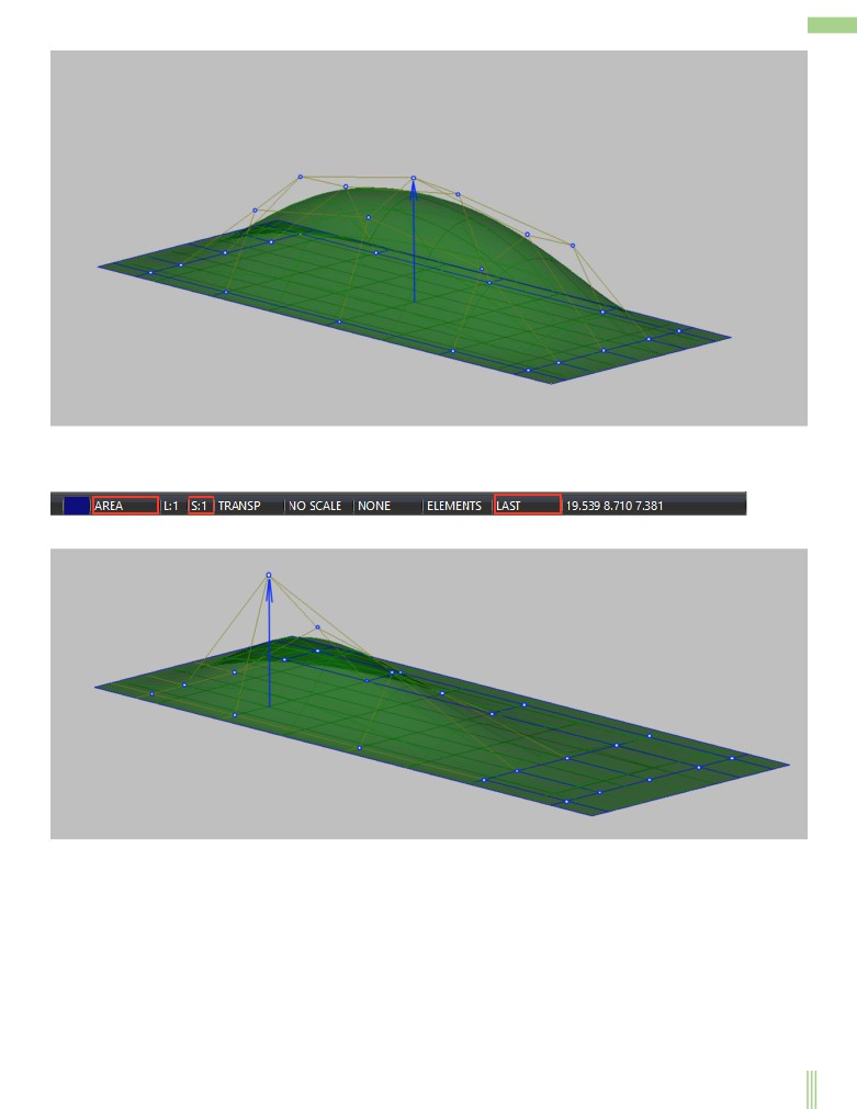
9 - This field shows the selected mode of model modification. There are three modes of model modification:
-ALL - model modification mode in which all control points of a line or a surface are changed depending on boundary points or
boundary lines,
- DO NOT - Mode Model modifications in which only boundary points or boundary lines are changed,
- LAST - Modification mode at which all points except the last ones change. This mode allows you to save tangents at the edges of
lines and surfaces when modifying.
These modes are switched by pressing the left mouse button of this field.
10 - This field shows the current cursor coordinates of the work window. If you click the left mouse button in this field, you will see
the following dialog:
14
This is done for the convenience of frequently used editing mode dialog.
15
Concepts.
The main elements of the mathematical model are three-dimensional point, line and surface. The line starts and ends at the points.
Lines can be connected to each other in points, forming a closed contour. This contour is a base for Surface, lines are boundary lines
of Surfaces, points - Corner points Surface.
All components of the project, starting from the surface of the hull, decks, bulkheads and finishing with equipment, structural
elements and pipelines, are built based on this model.
To perform complex elements, such as rotation surfaces, radius fillets, surface fillets, driver control elements are used. Drivers are also
used to design pipes and profiles.
To organizing structure of projects elements, you can use blocks that combine different elements of a mathematical model into groups.
Each element belongs to a block, and only one block. Blocks makes the structure of sub blocks as a tree.
The system allows you to make changes to the project at any stage of design, and all necessary re-buildings of project components are
automatically.
The coordinate system of the object.
Work with the project is conducted in a cartesian coordinate system. The axis X Direction along the length of the vessel, the axle Y is
directed to the width of the vessel, the axle Z Height. The origin point of the coordinate system and the frames numbering are given
when the grid is set. As a rule, this depends on the coordinate system used in the industry. The program allows to use any coordinate
system.
Units.
The meter is taken as the unit of measure in the system. The user can enter values coordinates with arbitrary accuracy; The entered
coordinates are displayed in the query string with an accuracy of up 0.1 of a millimeter.
Some value (e.g. thickness of the shell plates) in the corresponding dialogs can be specified in millimeters.
16
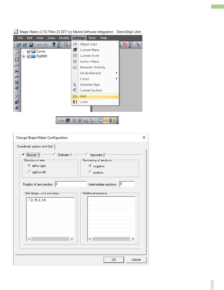
The coordinate grids.
The coordinate system of the object is defined by the grid definition. You can use the following command to open the Specify Grid
dialog box:
or from the toolbar Settings:
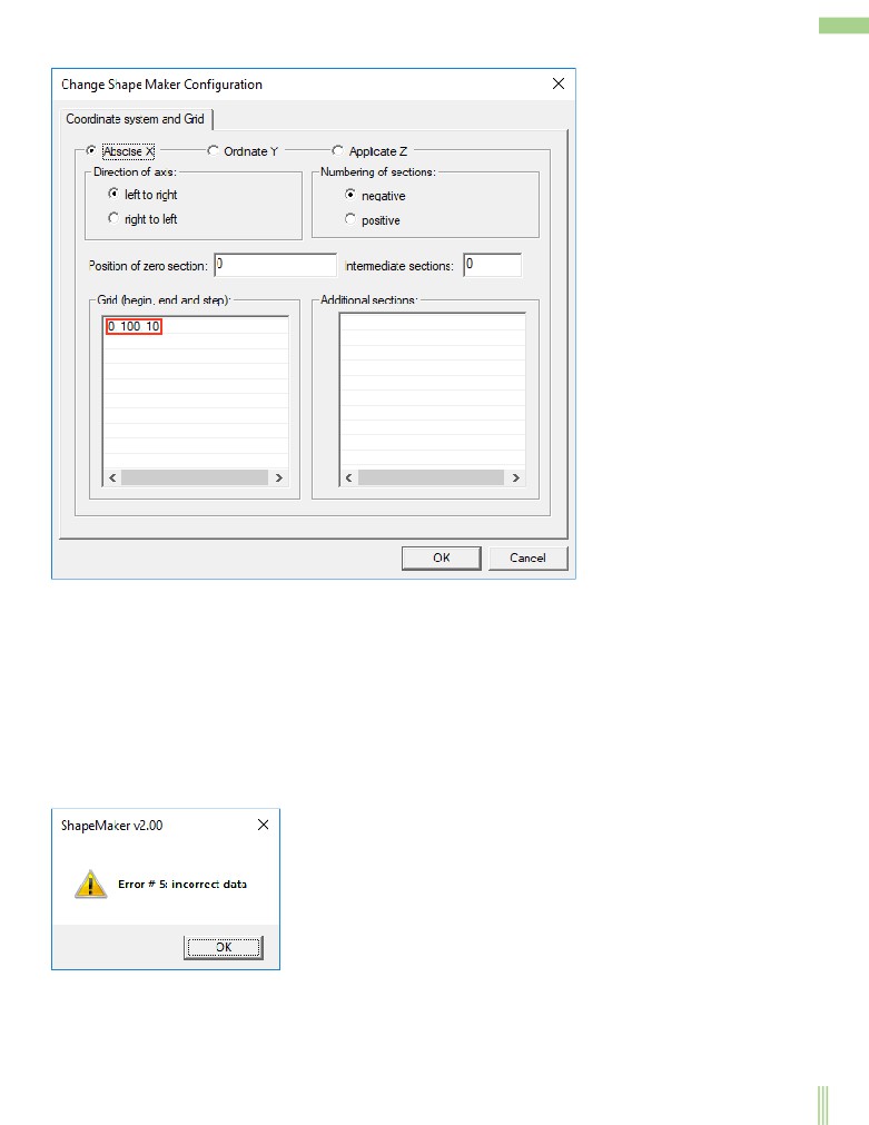
After you enter the command, a dialog box appears:
17
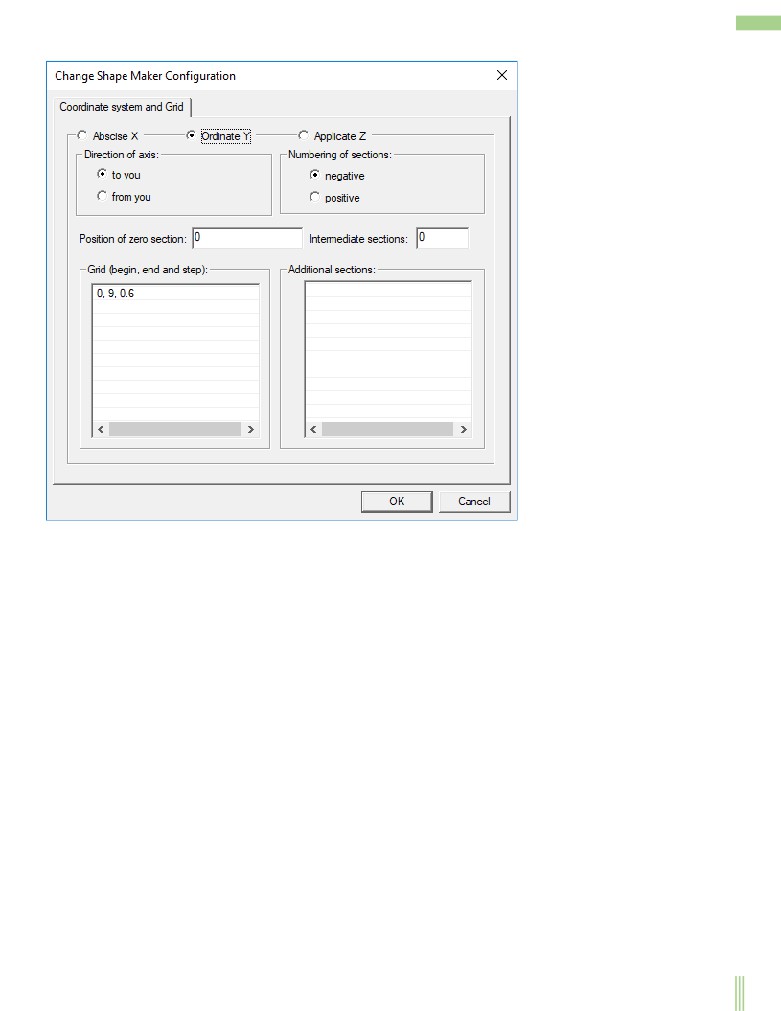
In this dialog box you can specify the direction of the coordinate axis, the origin of the coordinate system, Start section Position, Areas
with constant frames spacing and auxiliary sections, on each of the coordinate axes.
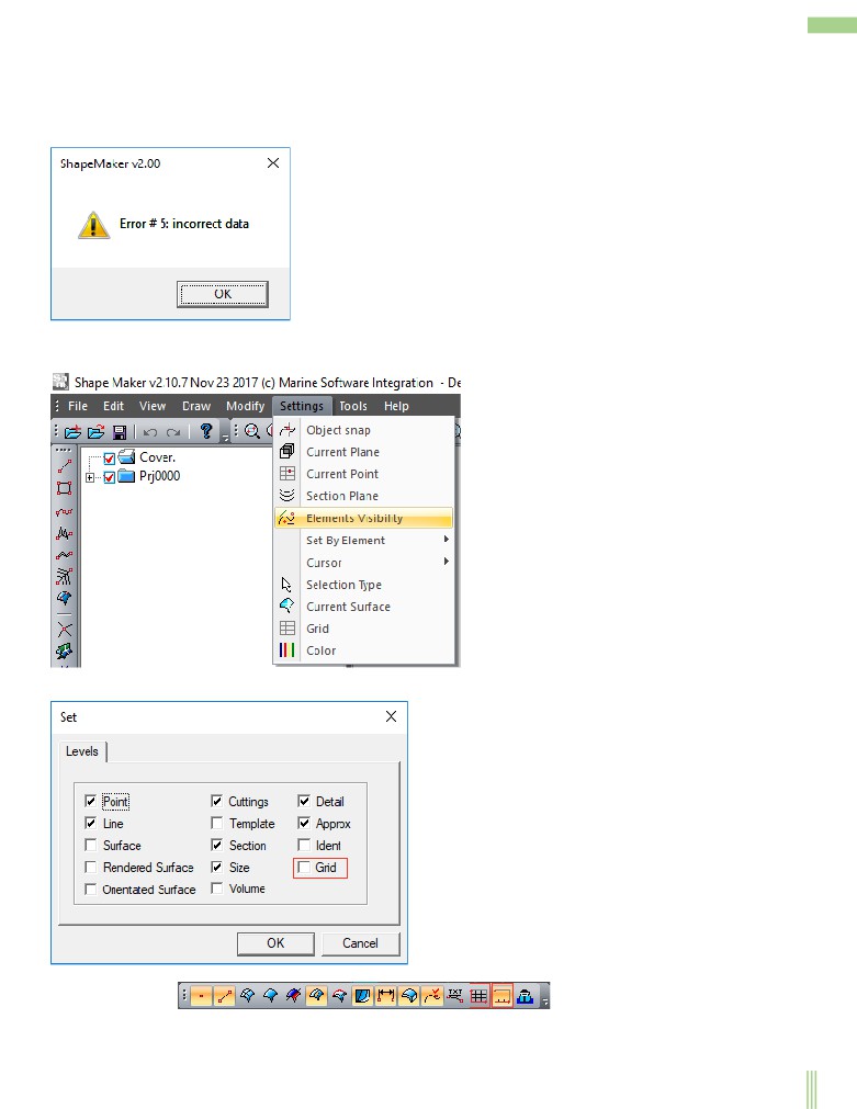
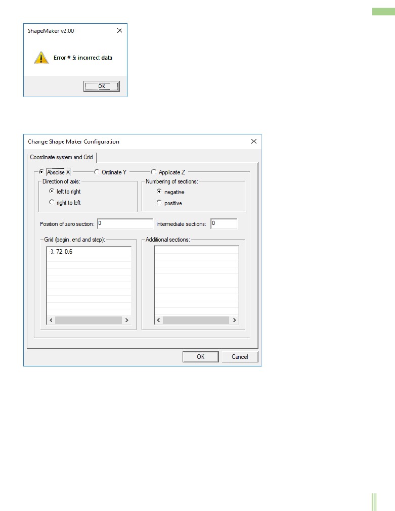
It is important to note that when specifying areas with a constant framer spacing the beginning of the next area must coincide with the
end of the previous area, and the number of frame spacing should be exactly the length of the area, otherwise the program will issue
the following message:
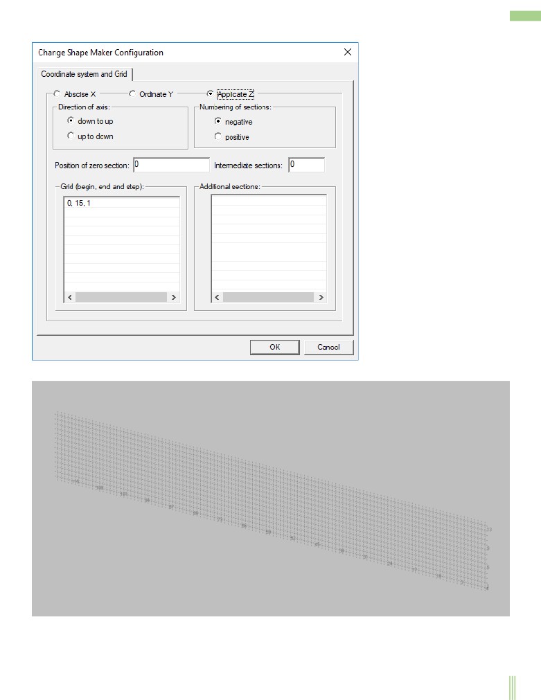
If the data is set correctly, then after pressing the button Ok The program updates the grid and the model coordinate system. If the grid
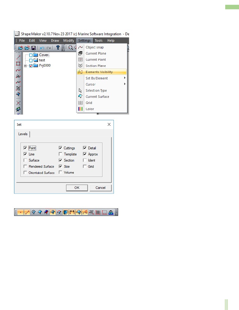
is not visible on the screen, you can visualize it using the following command:
After you select the command, the following dialog box appears:
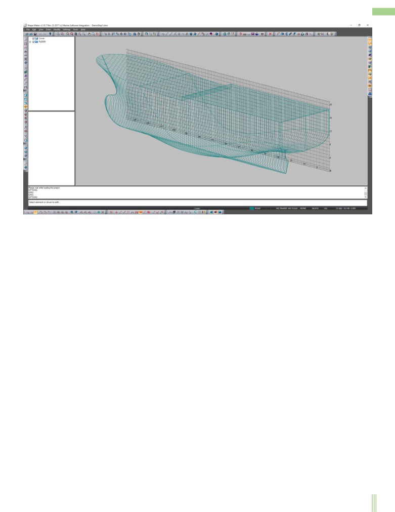
In which you need to choose render the item Grid. Another, And the simplest way to visualize the grid is select the appropriate item in
toolbar button Levels:
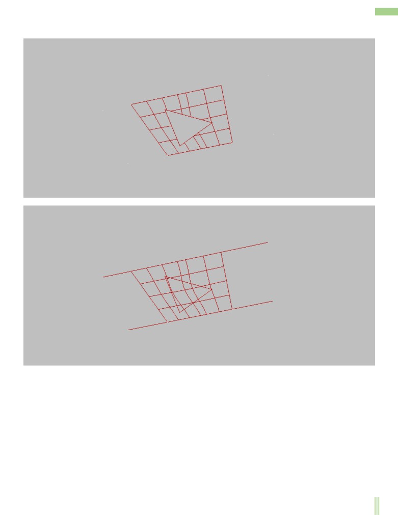
In this case, the program allows you to visualize one of the two grid visualization options this actual grid and scale with frames
numbers. Selected Toolbar visualization modes Levels highlighted. The following example shows a grid visualization.
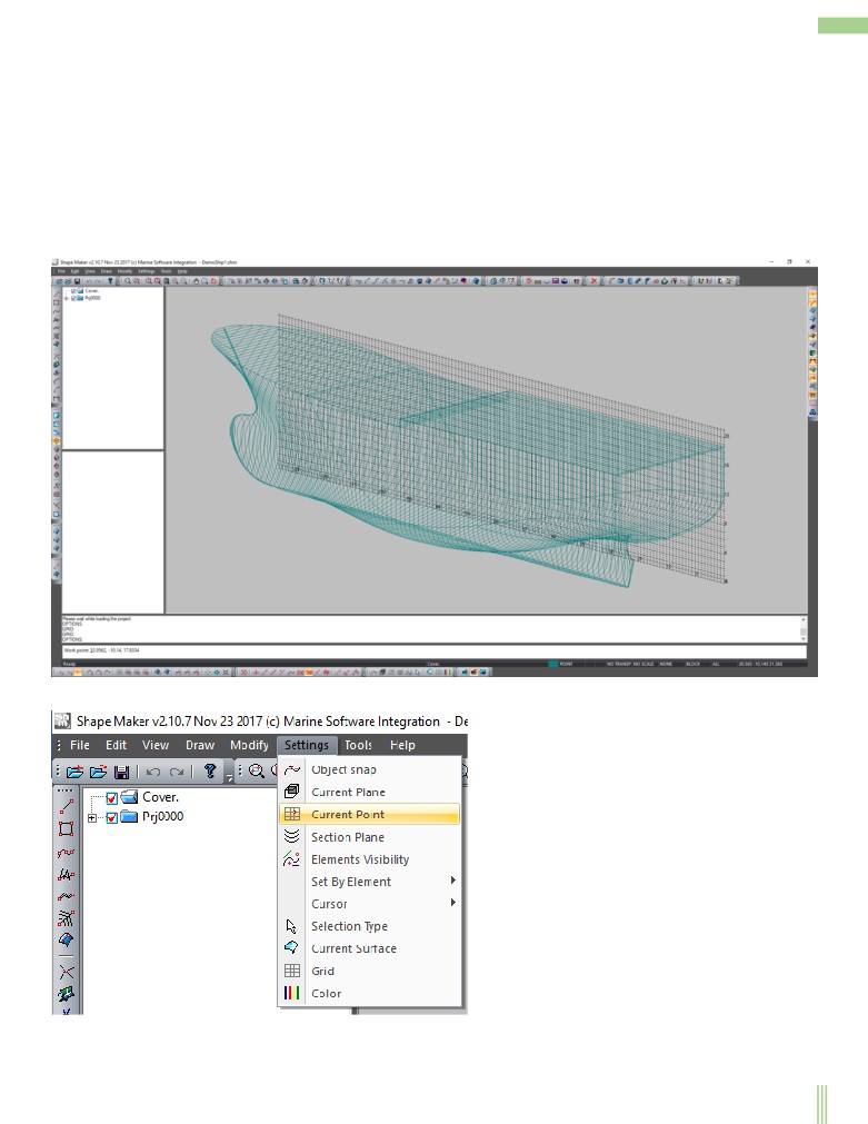
19
Work plane.
The mathematical model is three-dimensional. But when you enter a point from the screen, you can specify only two coordinates. For
third coordinate definitions work plane is using.
In general, in isometric, the work plane is always parallel to one of the main planes or the plane of the screen. In views Front, Side or
Plan The work plane is parallel to the corresponding main plane and to the screen plane (if isometric projection is not set).
The work plane always passes through the work point. By controlling the position of the work point, you can control the position of
the work plane at the depth of the current projection.
Will call the depth of the work point is its coordinate along the axis perpendicular to the work plane. On projections Front, Side or
Plan this will be the coordinate along the axis directed "In the depth of the screen". In an isometric projection, the work plane is
showing on the screen as a grid on the work plane. When you change the depth position of a work plane, the grid changes its depth
position. This is clearly seen in the isometric projection.
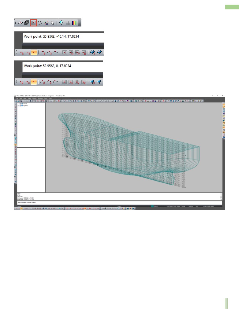
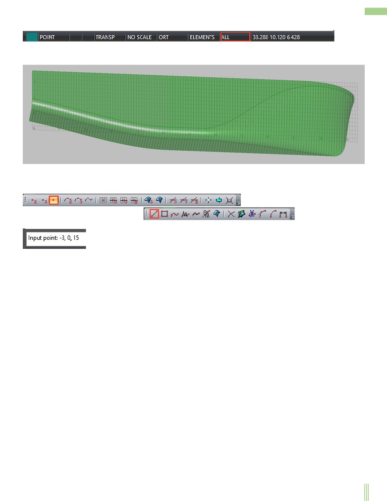
The following illustration shows the current position of the work plane on the projection Side
You can change the position of the current point by the following command:
20
You can also click the command to change the position of the current point from the toolbar Settings:
The new position of the current point is entered in the coordinate input window.
Change the position of the current point so that the coordinate Y was equal to zero:
Once the coordinates have been entered, the work plane will change its position and be in the vessel's center plane.
21
As mentioned earlier, the work plane always passes through the work point. The work point always takes the value of the last input or
modified point. Therefore, the work plane always matches the projection with the current depth of the entered point. This allows you
to specify, for example, polylines in different planes without interrupting the input, changing only the position of the current plane. As
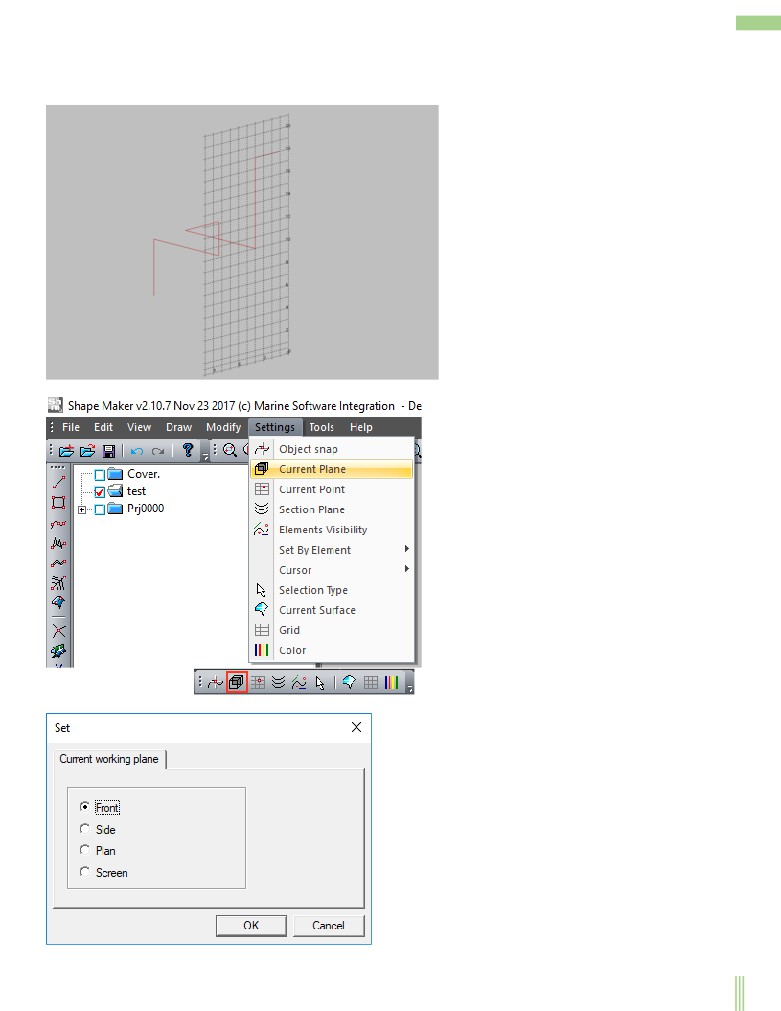
shown in the following illustration:
You can change the current work plane by:
or from the toolbar Settings:
After you select the command, the following dialog box appears:
,
where the user can change the current plane.
22
The sections plane.
To visualize surface sections, use the concept of the current sections plane. Typically, on orthogonal projections, the cut plane is the
same as the work plane. Thus, on the projection Side presented buttocks on projection Front frames, and on the projection Plan -
waterlines. When you visualize a model, only the sections defined by the sections plane will be displayed in the isometric. You can
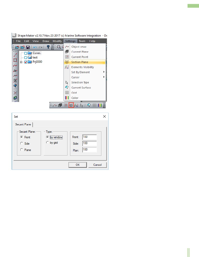
change the section plane by clicking one of the main projections Front, Side, or Plan, or by using the command:
or from the toolbar Settings:
After you select the command, the following dialog box appears:
You can change the sections plane by selecting one of the projections. The program also provides a selection of sections to visualize
the depth of the window or the depth of the selected volume and the grid. This will be discussed later.
23
Model projection.
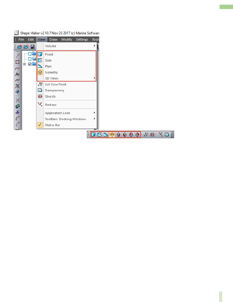
The program does not foresee the presence of separate windows for different projections of the model. Switching between different
projections of the model is performed by one of the following commands Front, Side, Plan, Izometry или 3D Views:
,
or by pressing a button from the Toolbar View:
When you click one of these buttons, one of the orthogonal projections or one of the isometric views of the model is displayed in the
work window.
Controls the visual representation of the model.
Zooming of the image on Projections Front, Side, Plan is carried out using the mouse wheel.
You can shift the image by changing the cursor position when the mouse wheel is pressed. In addition to this on the 3D Views You
can rotate the 3d model by moving the cursor with the CTRL button and the mouse wheel pressed at the same time.
24
The presentation of model elements.
The model consists of points, lines, and surfaces. You can change the appearance of the model in the work window by using the
following command:
After you select the command, the following dialog box appears:
Selecting the required items in this dialog and clicking Ok, you will give the program command to change the model view on the
screen.
It can also be done by pressing the corresponding button from the Toolbar Levels:
Let's briefly discuss the different models visualization options:
Points.
The points in the model are represented as line’s ends and surface corners. Sometimes bright dots interfere with the correct perception
of the shape of lines or surfaces. A large accumulation of points also prevents the whole model from perceiving. By turning off the
option Point in the dialog box (see above), you turn off the visualization of the points in the Model work window. It is important to
note that if the point is turned off for visualization it cannot be selected by the cursor editing mode.
Lines.
The line is visualized to the work window if the dialog box includes the option Line. Note that lines can be rendered in whole or in
part. If the dialog box includes the option Cuttings, only the untrimmed lines or part of the lines left behind the trimming will be
shown. If this option is off, the line is always shown entirely. If the line is turned off, it cannot be selected for editing.
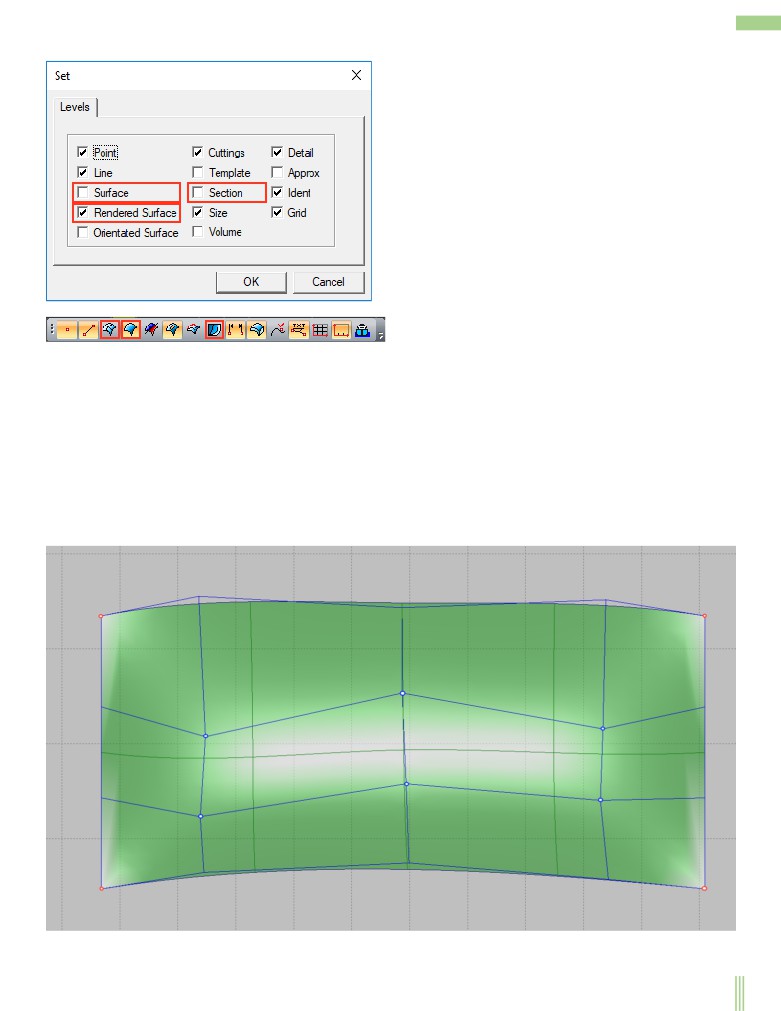
Surfaces.
Surfaces can be represented as a grid of an equal parameter line (Surface), as a set of orthogonal sections of this surface (Sections), a
shaded surface (Rendered Surface), as well as a surface view indicating the orientation (Oriented Surface). The orientation of the
surface is shown by different color of the outer side - red and the inner side - blue. Also, as in the case of lines, surfaces can be shown
trimmed and untrimmed depending on the option Cuttings. The surface can be selected for editing always even if all views of the
surface are turned off.
25
All other visualization options are not representing at not of interest at this time and will be considered later. Below is shown
Presentation of trimmed surface:
and untrimmed lines and surfaces.
26
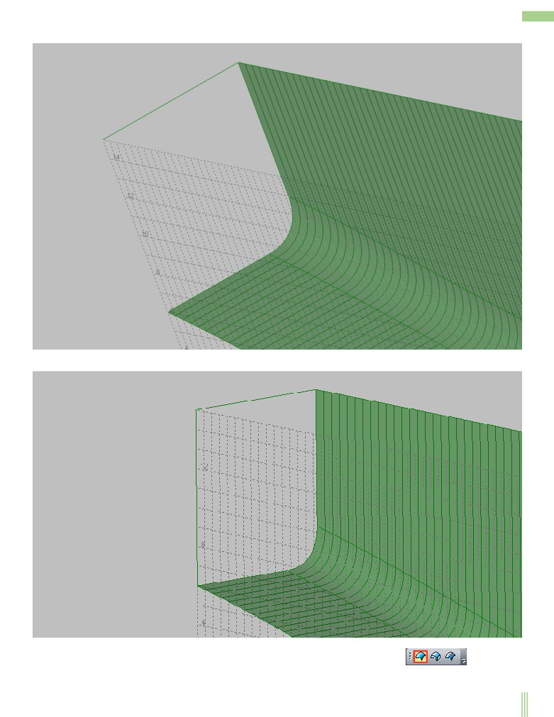
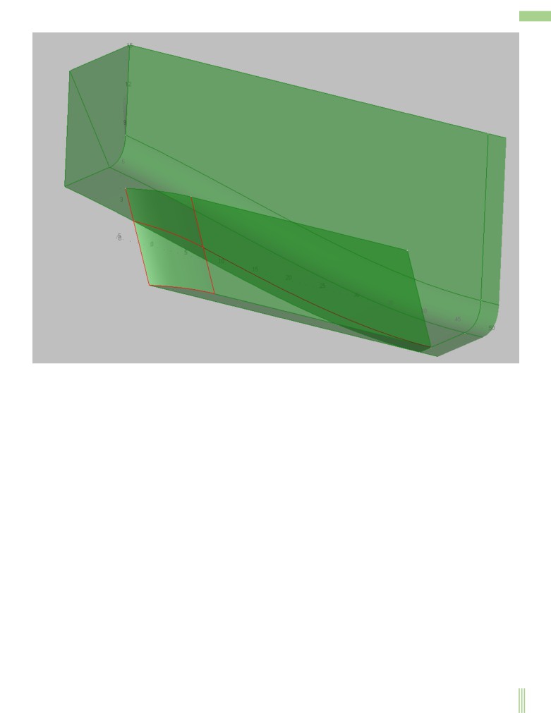
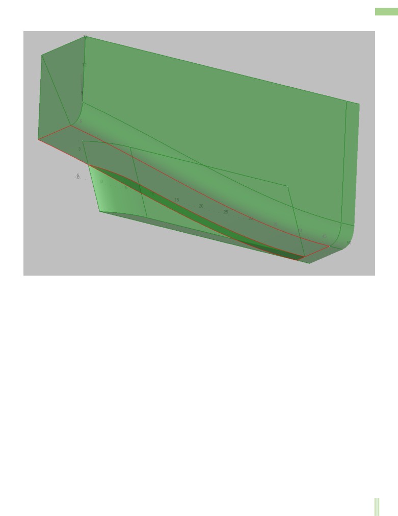
Visualize the model's working volume.
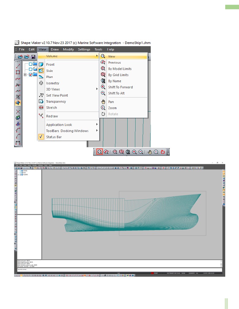
As a rule, smoothing of the ship’s surface make separately by fore and aft ship. On the projection Front both the lines and sections of
the fore and aft ship will be visible. This is a certain inconvenience. To quickly select the area in which the user is going to work and
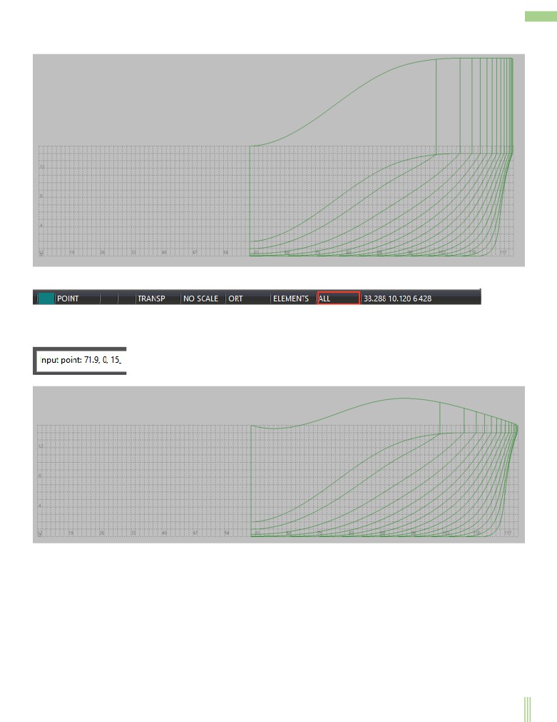
provides a simple tool to select the working volume of the model. So, to select the for ship is enough on the projection Side select fore
ship area by window with following command:
,
or by pressing a button from the Toolbar Volume:
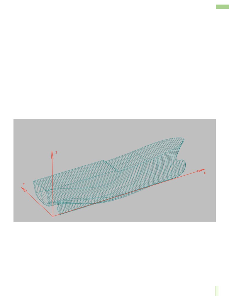
and select the desired area of the model.
In principle, this is very similar to increasing scale of visualized objects by selecting a window with the only difference, which in this
case is selected 3D volume. This is easy to see when you switch to one of the isometric views.
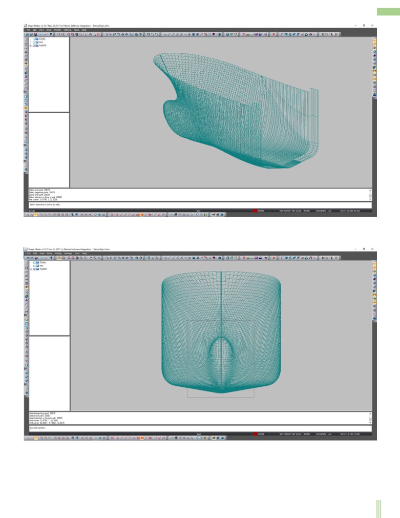
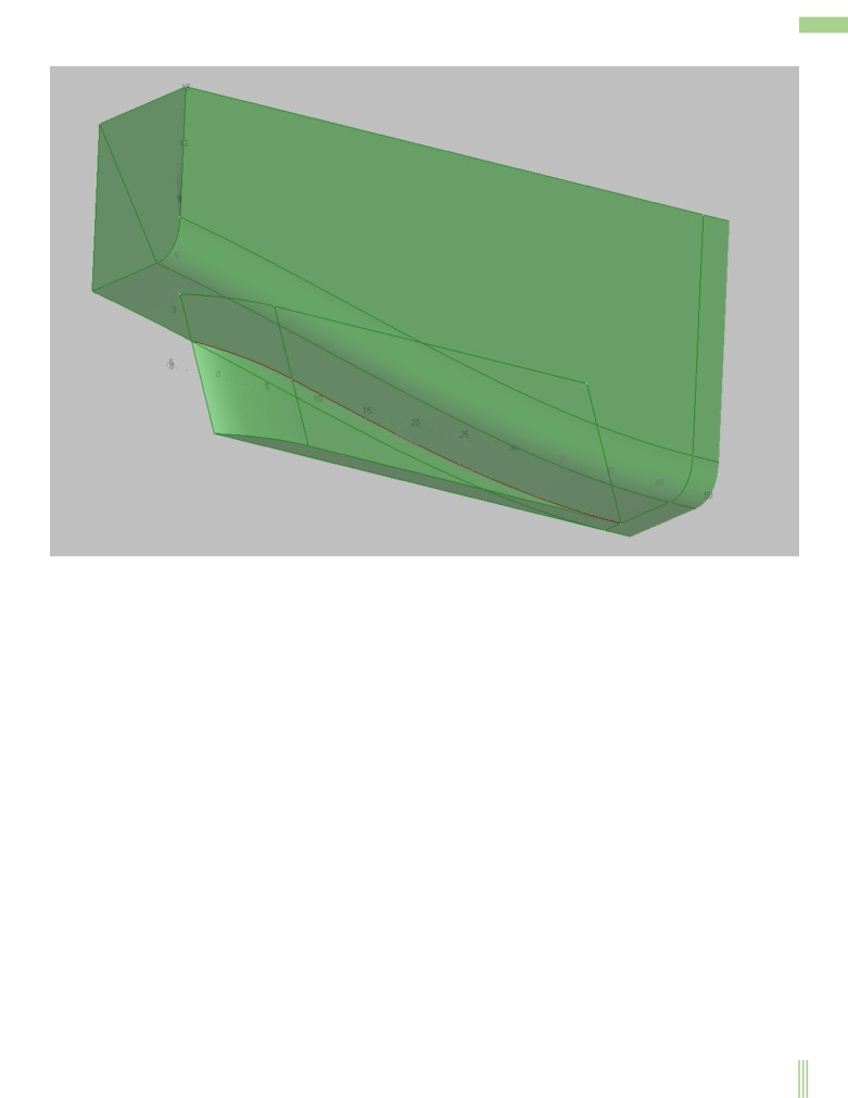
27
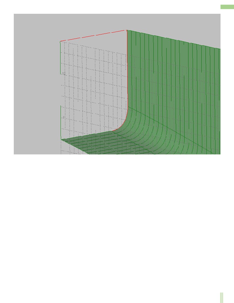
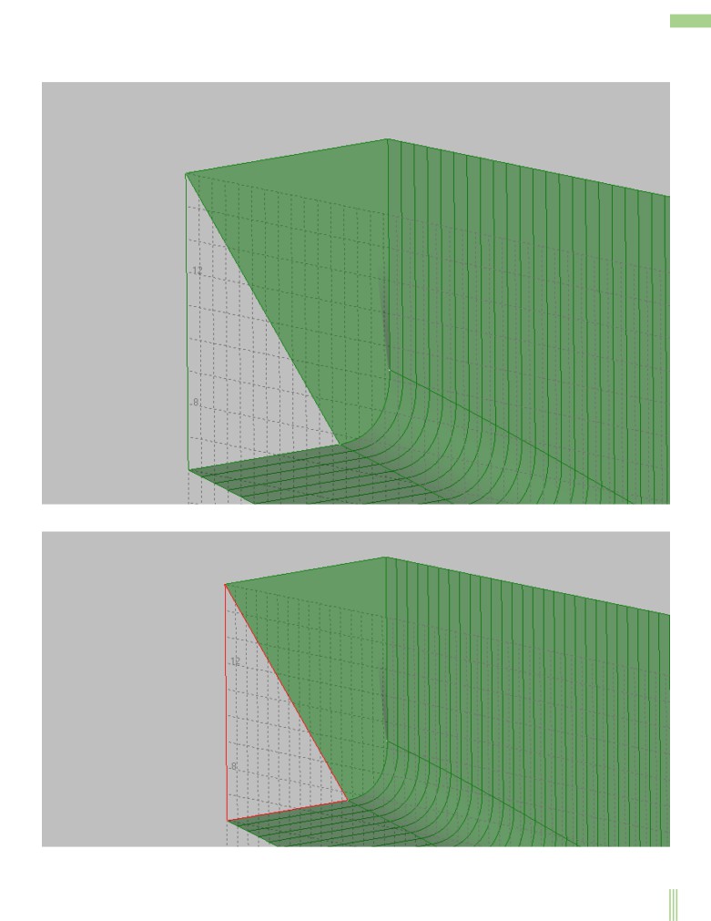
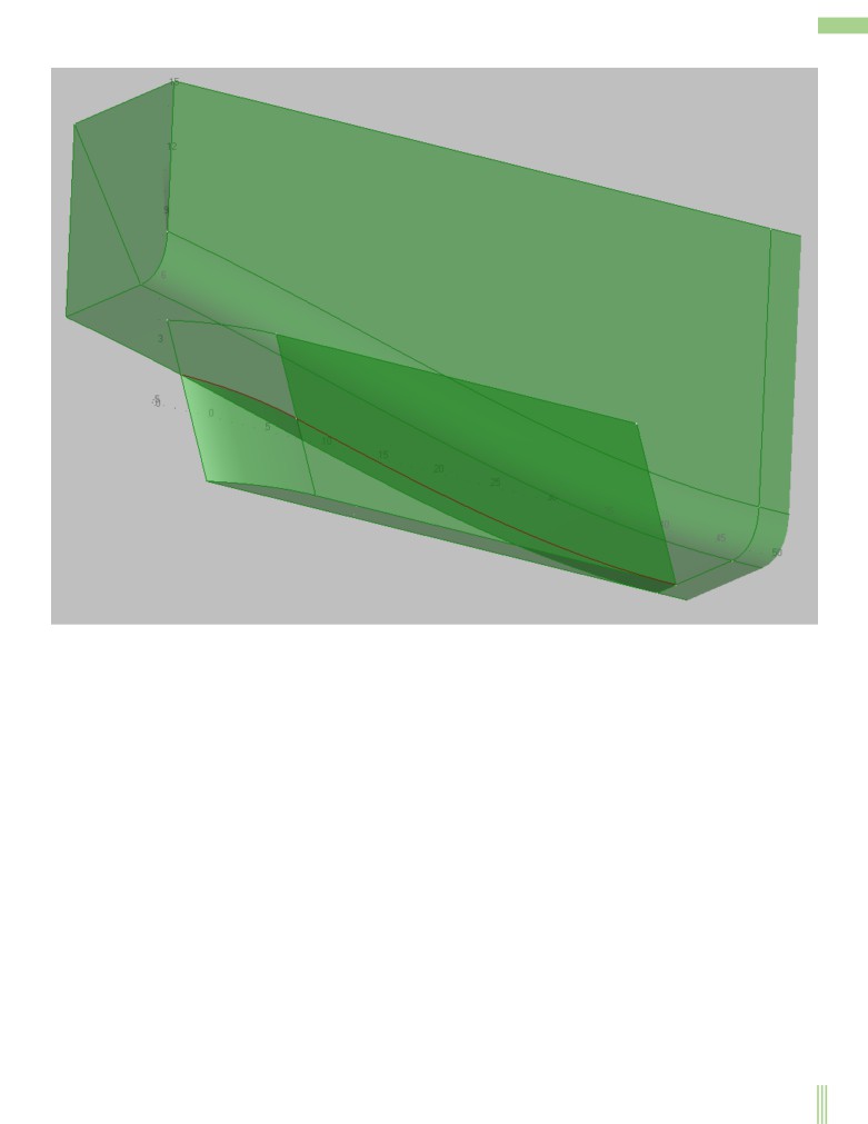
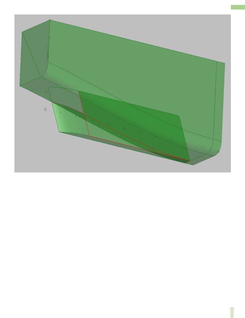
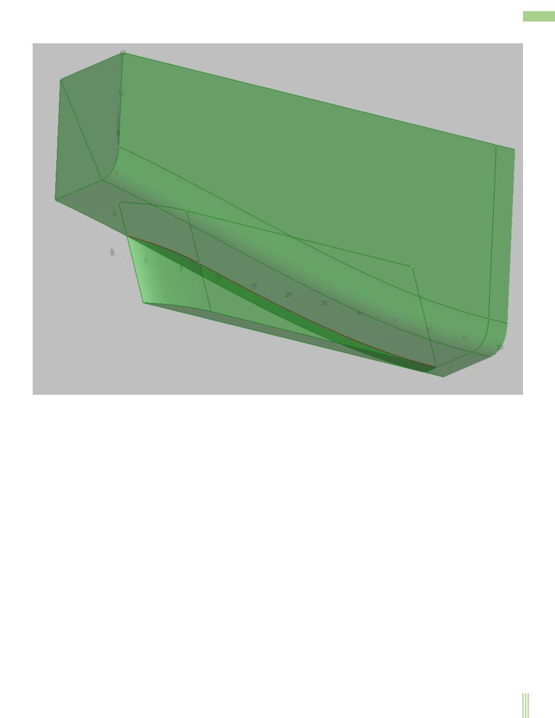
The visualized area corresponds to the selected volume window frame. All objects that do not inside this volume will be hidden. This
allows you to work more comfortably with the selected area. So, the lines and surfaces, that are in the aft ship will not interfere with
the fore ship objects. The window selection process can be repeated an unlimited number of times and on different projections.
The resulting volume will look like this.
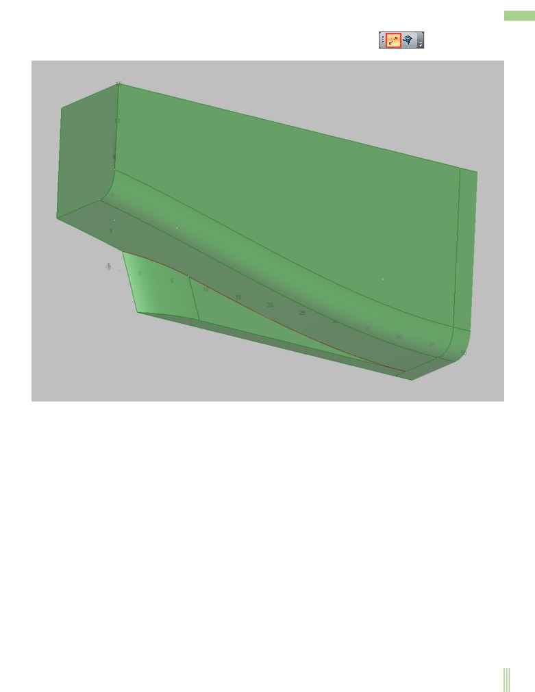
28
The program has a whole set of commands to work with the volume. Among them-to return to the previous volume, to set volume on
object dimensions, to set volume on dimensions of a grid and others. For a better understanding of these commands, please refer to
the user manual.
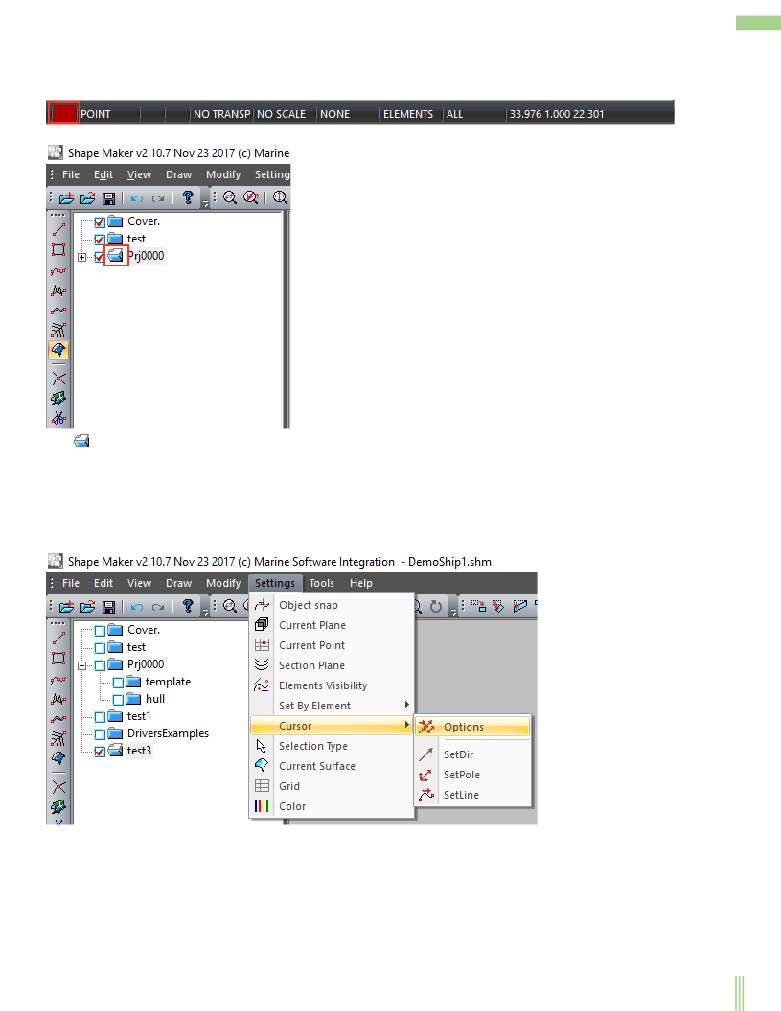
The visibility of objects in the block tree.
Each object in the model belongs to a block and only one. All the project blocks are organized as a tree. Each block has a specific set
of properties that allows you to control the visibility of the objects contained in that block.
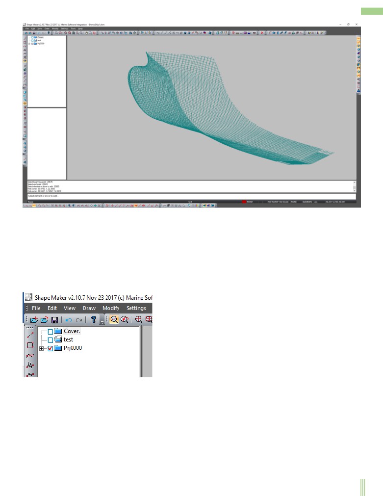
The simplest thing you can do to hide the elements of a block is to disable the block visualization. The example below shows that
only the elements contained in the block Prj0000 are visible at the moment, Elements of other blocks are hidden.
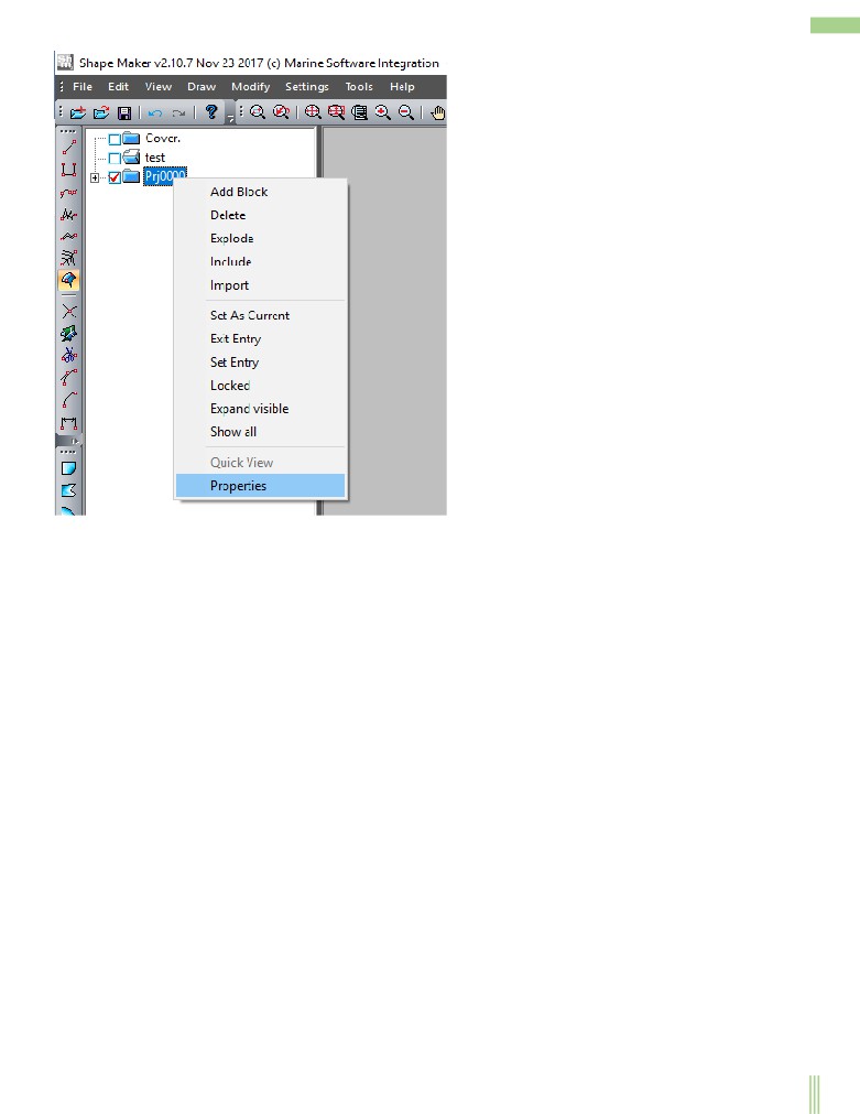
Another way to control the visibility of objects is to change the properties of an object in a block. To do this, just right click on the
desired block in the tree and, from the drop-down context menu, select the following command:
30
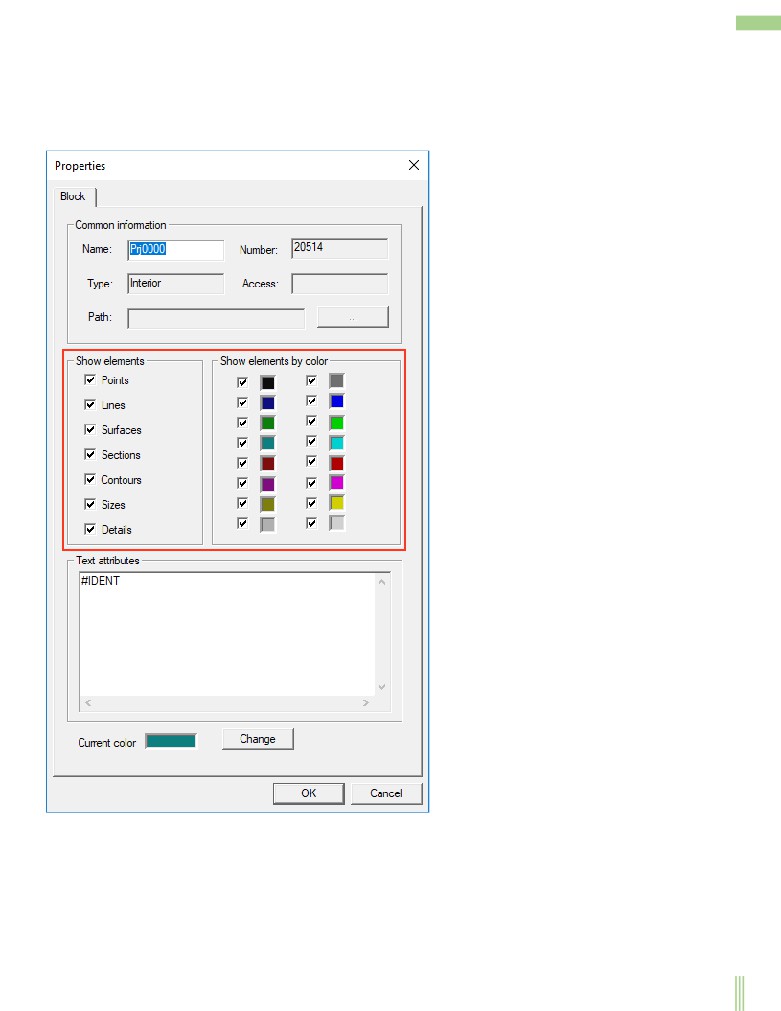
Appeared her as a result of this command dialog box allows you to change the visibility of objects that are in block. As you can see
from this dialog, you may want to show or hide specific types of elements or elements that have a specific color.
31
Select items to edit.
If no command is currently running, the system is in edit mode. To start editing an item, just click the item in the work window. If the
cursor capture area has multiple elements, the search is carried out among the visible elements that inside the current window in the
following order: points, cut-outs on lines, lines, dimensions, cut-outs on surfaces, sheets, surfaces.
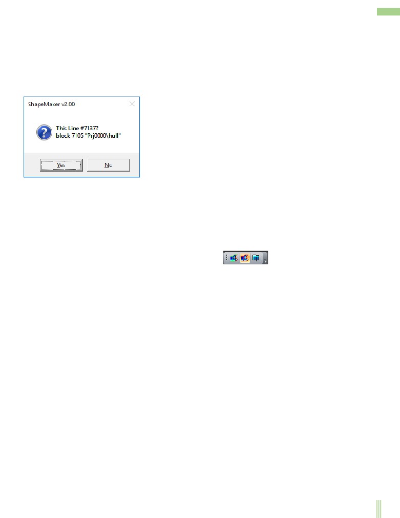
If there are several similar elements in the capture area, the system will ask you which item to select each time.
The last entered element will be offered last for editing. After selecting an item for editing, you will see either a control polygon, in
the case of a line or control polyhedron, a surface case. You can edit other items by editing the item settings dialog box.
It is important to note that to select a surface it is enough to click in the inner area of boundary lines of surface.
Select a group of items.
Sometimes you need to select a group of items for some commands. In this case, the following options are provided: Single item
selection, select by window or frame, select block from a tree of blocks, select block by specifying the element that owned the block.
Switching modes selection is done by pressing buttons of toolbar Selection:
. It should be noted that the elements
selection is combined with the selection of elements by a window or a frame. In the case when none of the elements gets the cursor,
the selection mode of the window or frame is turned on by a single selection of elements.
Specifies the outline of a lines set.
To specify a set of lines, you must sequentially specify the lines in the line in the desired order. The indicated lines are marked with
red color. To complete the instruction, press Enter. Press Esc Causes the markup to be canceled sequentially and then to cancel the
command.
If the lines must form a topologically linked chain or meet other conditions, the search is conducted only among the appropriate lines.
If the specified line does not meet the criteria, a message is displayed, and you are prompted to repeat the instruction.
Specify the start and end points of the chain to indicate the line chain. The system then automatically detects the closed chain. Lines
included in the chain are marked in red. If more than one chain can be built from the starting point to the endpoint ("Forks"), the next
line of the chain associated with the marked lines of the chain should be specified on the system's request.
In some cases, you use an option to specify the line chain by specifying all lines sequentially (like specifying a line set).
To specify a path, select one of the lines in the path. The system then automatically detects the closed loop. Lines included in the path
are marked in red. If these lines can form more than one contour (there are "forks"), you should specify the next contour line
associated with the marked lines on the system's request.
32
The current block and color.
The system uses the concept of the current block and the current color. All new items are entered the current block. The current color
is "painted" by the input elements. The easiest way to change the current color is to change it from the status bar.
,
In order to make the block current enough click the left mouse button on the block icon in the block tree.
Icon
Shows the current block in the tree.
The current block can be turned off and all input elements will disappear from the screen immediately after the input is completed. It
may be confusing at first.
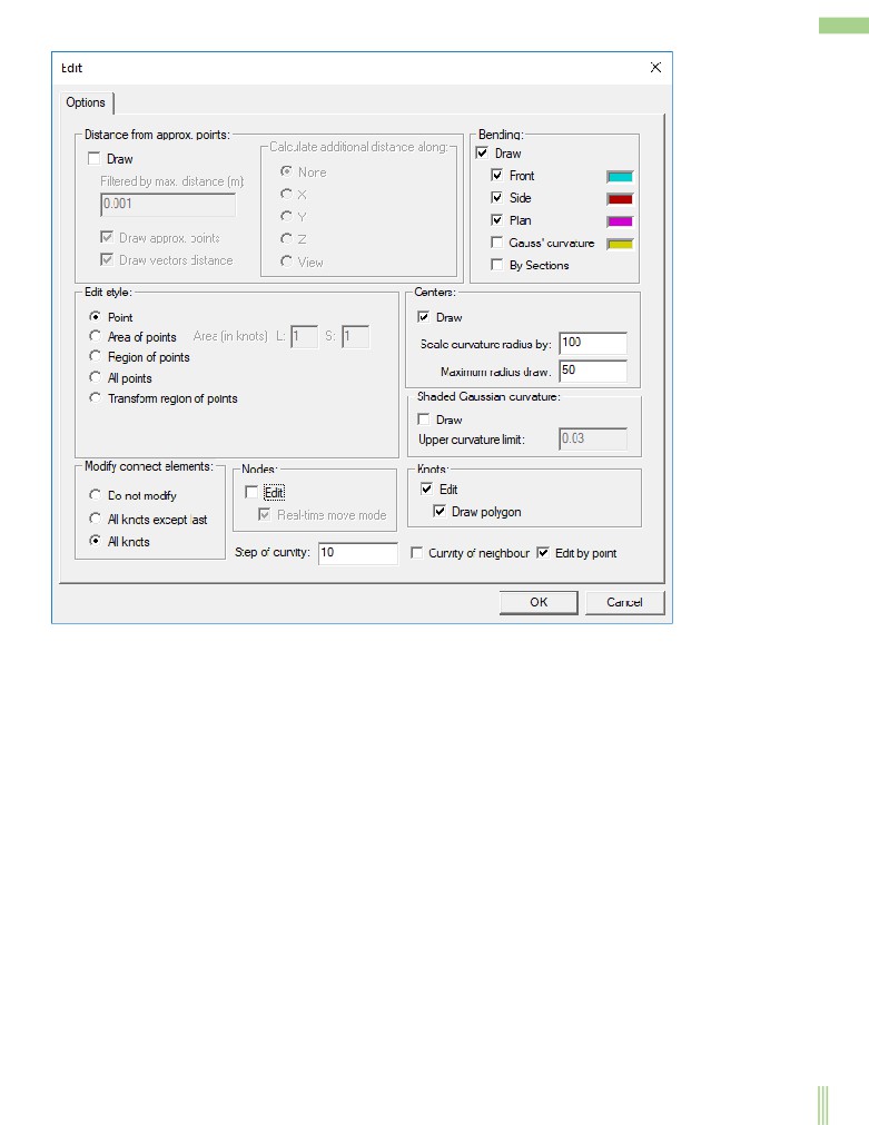
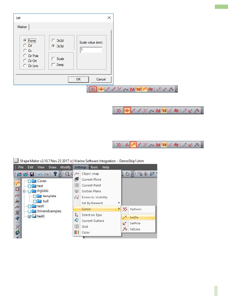
Cursor modes.
Different cursor control modes are used to make the builds and object snaps easier to perform. You can set the current cursor mode by
the following command from the menu:
The following dialog box will appear on the screen:
33
or by pressing a button from the toolbar Marker:
Let's look at the most common use of cursor mode.
Moves the cursor in a horizontal or vertical direction.
This mode is set by pressing the following toolbar button Marker.
This mode allows you to move the editable point vertically or strictly horizontally on the work plane. If you enter new lines, this mode
allows you to build a vertical or horizontal line. Horizontal or vertical is determined by the angle between the start point and the end
position of the cursor on the work plane.. If the angle is greater than 45 ° The vertical line is constructed, if less-horizontal. You can
also turn on the orthogonal motion mode with the hot key F10 and turn off the hot key F9.
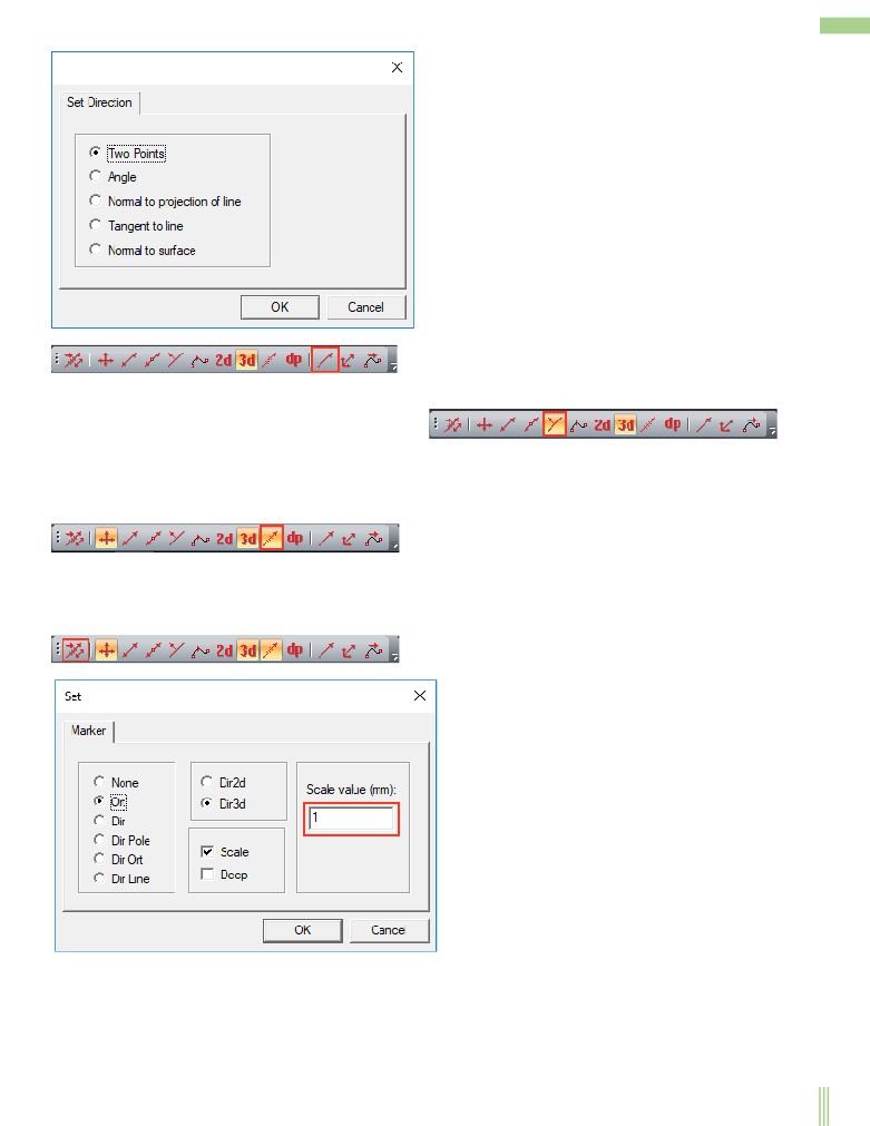
Moves the cursor in the specified direction.
This mode is set by pressing the following toolbar button Marker.
In this mode, the end point of the cursor will always be projected onto the line lying on the work plane and formed by the starting
point and the specified inclination angle. The inclination angle is set by the following command:
The dialog box selects how to set the angle:
34
The same dialog box can be accessed by pressing a button from the Toolbar Marker.
Move the cursor in the orthogonal direction to the given angle.
This mode is set by pressing the following toolbar button Marker.
This mode is practically no different from the previous one. The only difference is that the movement occurs at an angle perpendicular
to the preset.
Scaled move the cursor in the specified direction.
This mode is set by pressing the following button of toolbar Marker.
Scaled cursor movement is used if you want to move the point a very short distance in the specified direction. As a rule, this mode is
used when smoothing curves and surfaces. When you select a moving point, the rubber line with marks is displayed. The direction of
the rubber line shows the direction of the point movement and the number of tick marks shows how the conditional units are moved
point.
You can set the unit size value by pressed following button of toolbar Marker.
and setting the desired value in the following menu.
The default value of the displacement unit is 1 mm.
Other modes will be discussed later. For a fuller study of the details, we recommend reading the User Guide.
35
Change the coordinates of the mouse point.
The system implements the option of changing the coordinates of the mouse in two clicks. The first click selects the point you want to
change. After selecting, the point starts to move after the cursor. The second click captures the new position of the point. This editing
method is used in all modes of the system.
36
Mathematical model.
The design technology of the hull surface when using this mathematical model is as follows. First, you enter the lines that make up the
spatial structure of the object. It can be buttock in CL, deck line, knuckle lines, midship section line. Then the surface is "stretched" to
this frame. Finally, the lines and surfaces are adjusted to get the desired shapes (the shape of the surfaces is controlled by the sections
of surfaces).
Point.
The point has three coordinates that determine its position.
Depending on the presence of topological relationships, the system presents different kinds of points:
-A spatial point is a point that has no topological relationships,
- Point on the line is the point that always lies on the line that is associated topologically.
- Point on the surface is the point that always lies on the surface that is associated topologically.
-The point of intersection of two lines is the point obtained as a result of intersection of two lines. Such a point cannot be changed.
-The point of intersection of a line and a surface is the point received as result of intersection of a line and a surface. Such a point also
cannot be edited.
Line.
The line is a smooth (twice continuously differentiable with respect to a parameter) parametric curve in 3-dimensional space. It is
represented as a heterogeneous cubic polynomial B-spline. This curve is represented as a set of Bezier segments that are cubic
parametric curves connected to each other at points called B-spline nodes. The number of Bezier segments in the curve is less than the
number of its control points by 3.
The position of any point on a line is determined by its parameter, which changes monotonously and continuously along the curve.
The direction is defined for the line, i.e. the beginning and the end are defined. The direction of the line is determined by its start and
end points.
1 - The end point,
2- B-spline control points,
3 - Control polygon,
4- The segment of the curve,
5- B-spline node.
B-spline is defined by a control polygon, which, by some rule, is mapped to a curve with the following properties:
- The polygon must contain at least four control points of B-spline (in the future we will sometimes call them bows);
- The start and end points of the curve are the same as the starting and ending points of the polyline;
37
- Tangent at the starting point of the curve is directed along the first segment of the polygon one, at the end point - along the last one;
- The curve tracks the shape of the polygon (in particular, polygon with the self-intersection corresponds to the curve with the self-
intersection; if all the vertices of the polygon lie on one straight, the curve will coincide with this straight);
- The curve is contained in the "convex sheath" of polygon, that is, the dimensions of the curve is known no more than the dimensions
of the polygon;
- Changing the position of one of the vertices of a polygon vertex results in a change of no more than four segments of the curve;
- Arc and circumference approximated with the maximum radial deviation from the true arc can be 0.1 mm.
From the user's point of view, the control polygon is a tool to correct the shape of the line.
The line relies on 2 points. A line that starts and ends at one point is not used and cannot be drawn. The line changes shape when the
position of the endpoints changes.
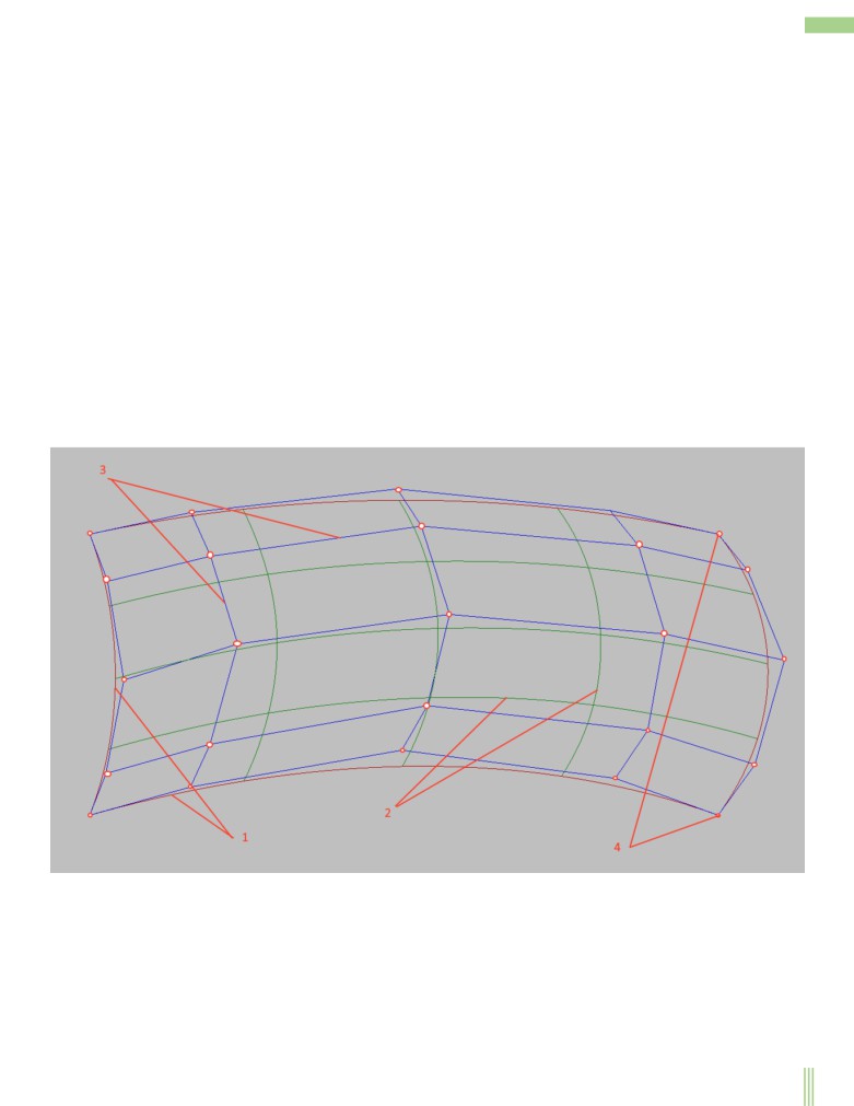
Surface.
The surface element is a smooth parametric B-spline surface. Her mathematics is similar to the mathematics of B-spline curve, with an
amendment to the 2d case.
The surface is based on 2, 3 or 4 boundary lines forming a closed loop. The closure is provided when the corner point of the surface is
common to the two boundary lines. The surface changes shape when the shape of the boundary lines changes.
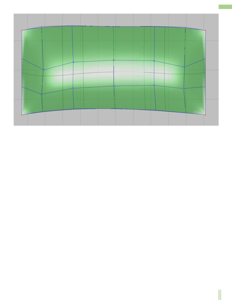
The representation of the surface shape gives lines of equal parameter and section. The shape of the surface can be controlled by
changing the shape of the boundary lines and the position of the surface control grid.
The number of nodes of the control grid of a surface and their arrangement is determined by the polygons of boundary lines. If the
opposite boundary lines have the same number of control grid nodes, the surface grid along the corresponding direction will have as
many nodes of the control grid. Otherwise, the number of nodes of the surface control grid along this direction can be increased, but
not more than the sum of the control grid nodes of the specified lines.
1- Boundary lines,
2-lines of equal surface parameter,
3-Control polyhedron surface,
4 - Corner points.
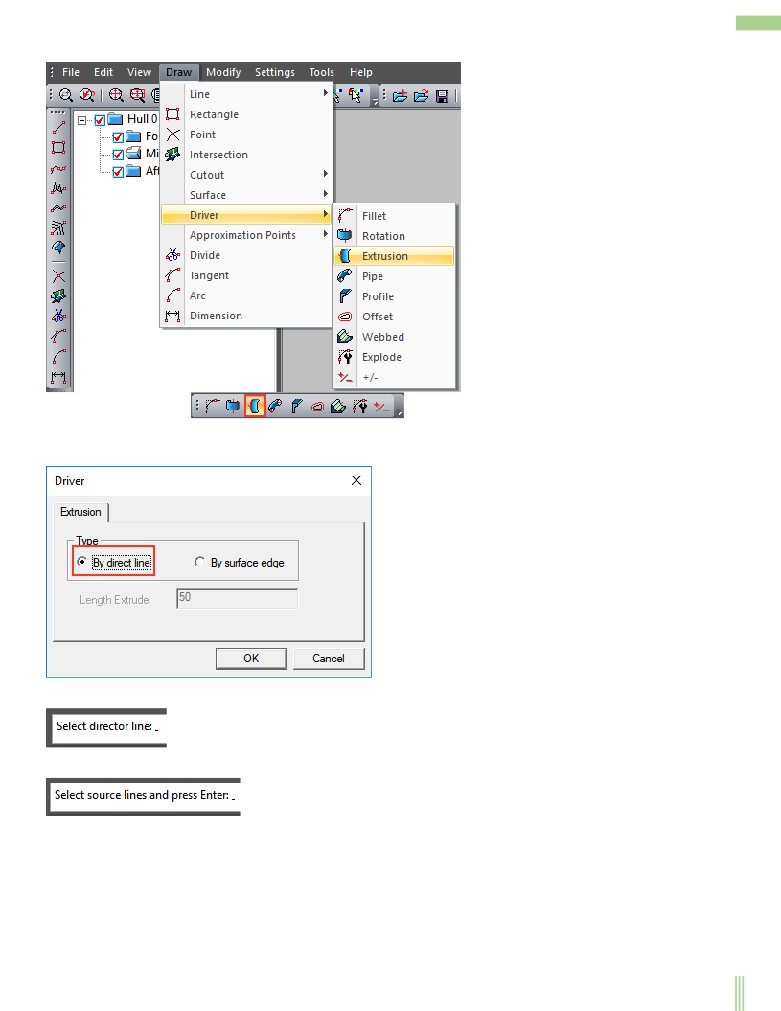
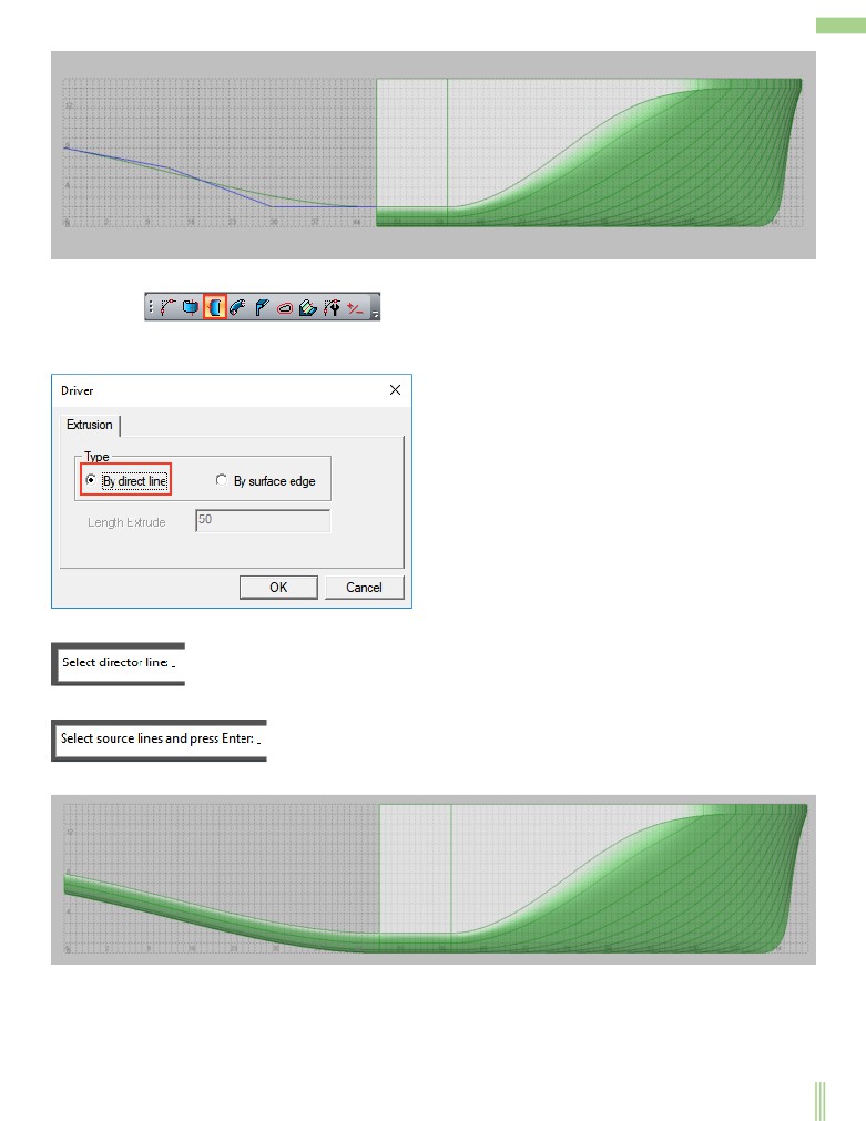
Driver.
The system implements complex constructions, such as the surface of rotation, filleting of lines with radius, etc., and their automatic
support during correction. The elements of the driver structure are no different from the usual elements. They have all the appropriate
topological dependencies and relationships among themselves. They can be used to construct other elements (lines, surfaces, etc.), for
38
object snaps (geometric and topological), as basic elements of fixation. The correction of driver's source elements or driver parameters
causes automatic rebuilding of driver elements.
Links.
As it was told Above, the line changes shape when the position of the endpoints changes, the surface changes shape when the
boundary lines change. This dependency is implemented through direct and backward links between elements. For example, a line has
direct references to its endpoints, and these points are backward references to the line, the surface has direct references to the
boundary lines and angular points, and the lines and points are the back references to the surface.
The element names.
Each item in the project database has its own unique number or name. This number can no longer be assigned to any other database
items, even if the item is deleted. Based on this, the links between elements is implemented. You can also use unique element names
to select an item to edit. In this case, instead selecting element by cursor in the working window, in the coordinate input line you just
need to type its name and click Enter. In this case, the item will be selected for editing even if it is in a disabled block. This property
is often used in cases where you need to understand the topological dependencies of one element from another.
The topological dependency of the elements.
We will call the topologically element dependent on another element (reference) if it has at least one common point with the reference
element, a direct reference to the reference element, and changes when the reference element changes. The topologically line is
dependent on its endpoints, the surface-from the boundary lines and corner points.
The topological relationship of the elements.
Topologically bound will be called two elements, if there is a topological dependency between them. Topologically the line, its end
point, its surface, its boundary line, and its angular point are linked.
Topologically related We will also call two elements if there is any common element for them, from which topologically depend on
these elements or which depends on these elements. Topologically are linked by two lines if they have a common endpoint.
Topologically are linked by two surfaces if they have a common boundary line or a common corner point.
39
Topologically the surface and the line that "comes" to the corner point of the surface are linked.
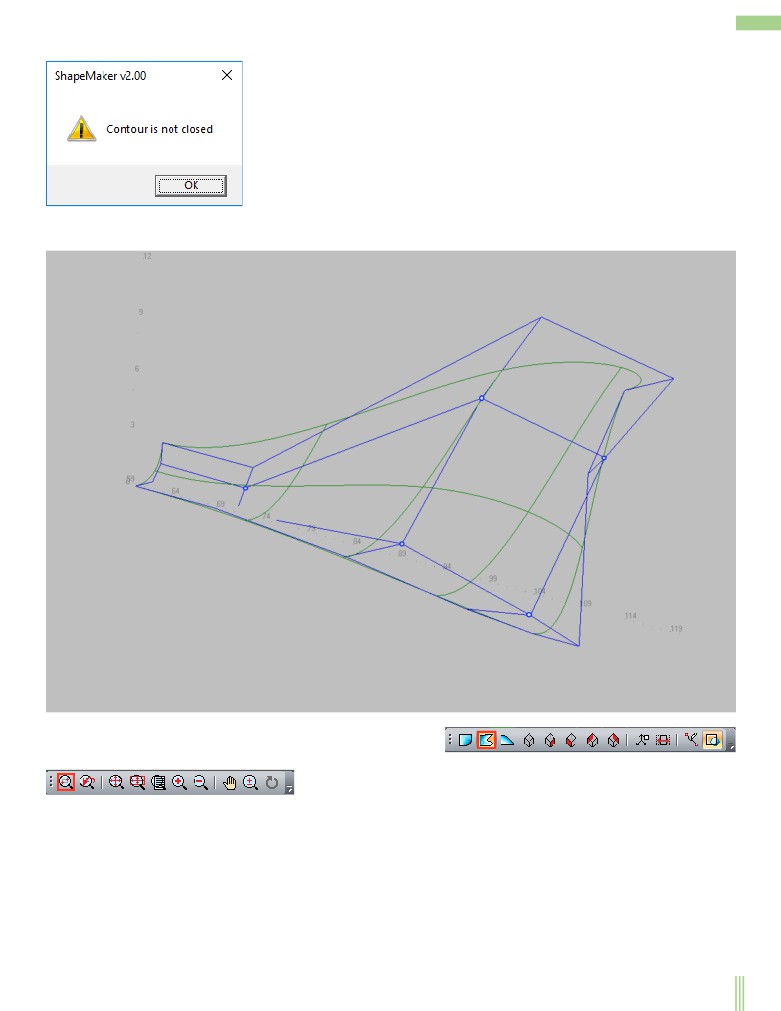
Thus, the reference contour for a surface will be closed if its lines topologically connected. We shall call such contour topologically
closed. In this way, the surface can only be set on a topologically closed loop. Two topologically lines are linked if they refer to the
same point. There is no topology link if the lines refer to different points, even if the points have matching Cartesian coordinates.
40
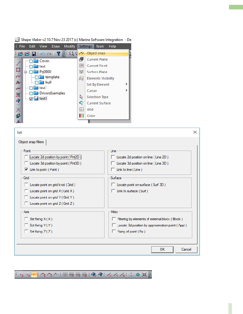
The object snap.
Object snaps allow you to use the geometry of other elements (anchor objects) When you enter points, such as a point on a line, a line
intersection point, a grid line, an intersection point of two grid lines, and so on. At the same time, object snaps serve as a means of
creating topology constraints in the model. You can set the desired snap mode by calling the appropriate command from the menu.
The result of this command is the following dialog box:
After selecting the desired object snap mode and clicking OK, we set the current binding method, That will be used when you enter
and edit items.
can also be done by pressing the corresponding button from the Toolbar Osnap:
. Note that some of the object snap filters can be
used together. Some are incompatible with each other. Consider how to work more frequently used bindings:
41
Snaps to a point by two coordinates.
The mode is selected by pressing the corresponding button from the Toolbar Osnap:
This binding mode is not topological. If you combine the cursor with one of the previously entered points, the new point will be
assigned the coordinates corresponding This point. The depth (perpendicular to the work plane) will be the same as the work plane.
For example on projection side coordinates X And Z will be the same as the previously entered point. Coordinate Y Will match the
work plane's coordinate value. If no point is in the capture area of the cursor, the snap will not work and the corresponding coordinates
of the new point will be the current cursor coordinates on the work plane.
Snaps to a point by three coordinates.
The mode is selected by pressing the corresponding button from the Toolbar Osnap:
This binding mode is also not topological. When you combine the cursor with one of the previously entered points, all three
coordinates of the point will be assigned to the new point. That is, geometrically the new point will coincide with the previously
entered. Note that in this case the position of the work plane will change according to the new coordinate values of the entered point.
If no point is in the capture area of the cursor, the snap will not work and the corresponding coordinates of the new point will be the
current cursor coordinates on the work plane.
Topological snap to point.
The mode is selected by pressing the corresponding button from the Toolbar Osnap:
This mode is similar to the previous one, and differs from it only in that establishes topological connection with the previously
entered point. For example, if you enter a new line instead of creating a new point for the end of a line, you specify a reference to an
existing point. That is, if a single point converges several topological related lines, all these lines have a reference to one common
point.
Snaps to a line by two coordinates.
The mode is selected by pressing the corresponding button from the Toolbar Osnap:
This snapping mode is not topological and works like a two-coordinate point snap mode. The only difference is that in this case the
coordinates of the nearest point on the selected line are taken. If no point is in the capture area of the cursor, the binding will not work.
Snaps to a line by three coordinates.
The mode is selected by pressing the corresponding button from the Toolbar Osnap:
This binding mode is not topological and works as a three-coordinate point snap mode.
In this case, the new point you enter will be assigned the closest point coordinates on the selected line.
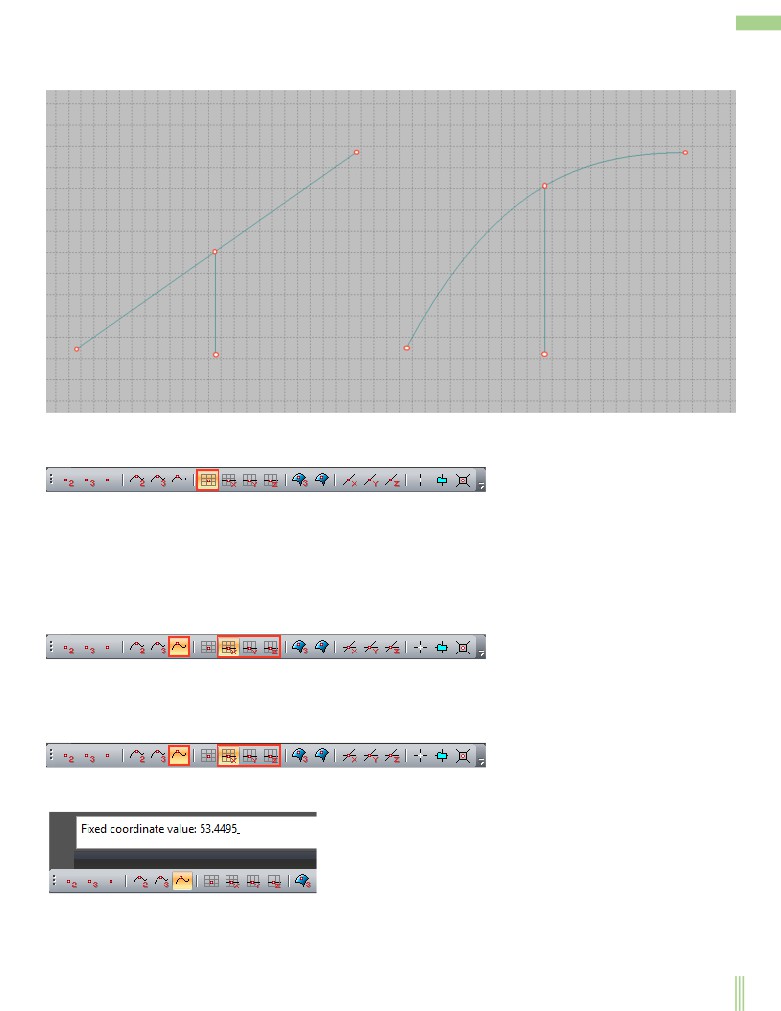
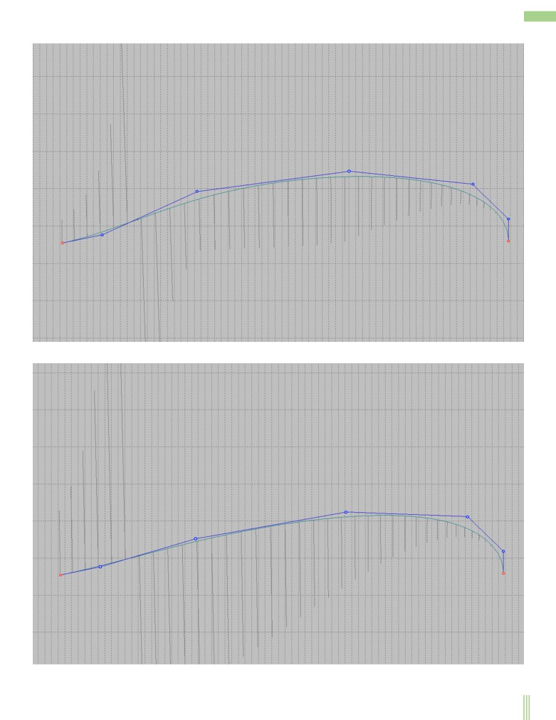
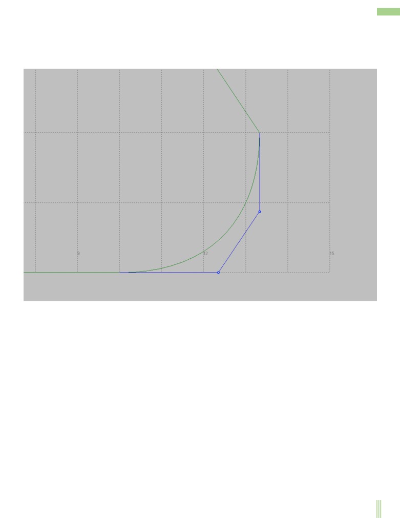
Topological snap To line.
The mode is selected by pressing the corresponding button from the Toolbar Osnap:
This mode is similar to the previous one, and differs from it only in that it sets the topological link to the line referenced by the point.
The essence of topological binding is that the point always follows the line when its shape changes. In order for the position of a point
on a line to be determined by a natural way, the fixation of one of the coordinates is used. When you snap a point to a line, you must
specify one of the coordinates X, Y Or Z.
If you use the orthogonal cursor mode when you enter or edit a point, the coordinate capture is automatic. Example of a topological
snap to a line with a coordinate fixation X (projection side is shown). Left-line before modification, right after modification. As you
42
can see from this example, the coordinates of the bound point are recalculated c By saving the coordinate value X Unchanged. The
vertical line remains strictly vertical
Snaps to a mesh node.
The mode is selected by pressing the corresponding button from the Toolbar Osnap:
This binding mode is not topological. When you combine the cursor with a grid node, the new point will be assigned the coordinates
corresponding Coordinates of the grid node. The depth (perpendicular to the work plane) will be the same as the work plane.
Note that all of the above modes can not be used at the same time.
There are several additional binding modes that can be used along with a line binding.
Snaps to the point of intersection of a line with one of the grid lines.
The mode is selected by pressing the corresponding button from the Toolbar Osnap:
Этот режим аналогичен топологической привязки к линии с фиксацией одной из линий сетки.
Snaps to a line with the exact job of one of the coordinates.
The mode is selected by pressing the corresponding button from the Toolbar Osnap:
This mode is similar to a topological reference to a line with the exact definition of one of the coordinates of a fixed point.
In this case, when binding, the system prompts you to specify the exact value of the selected coordinate.
All other binding cases are not of interest at this time.
43
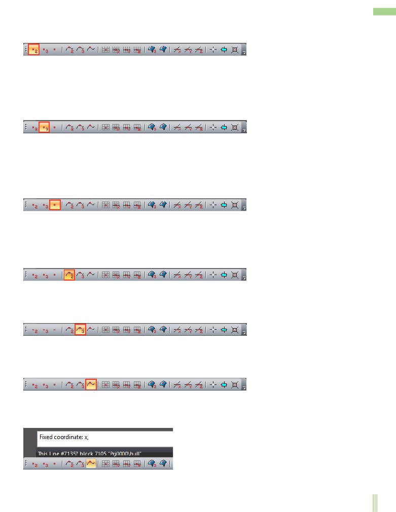
Working with lines.
The program uses three main types of lines: spatial lines, lines on the surface, and the intersection lines of surfaces. You can edit
spatial lines and surface lines. The surface intersection lines depend on the shape of the crossed surfaces and cannot be edited.
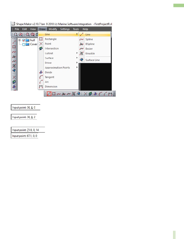
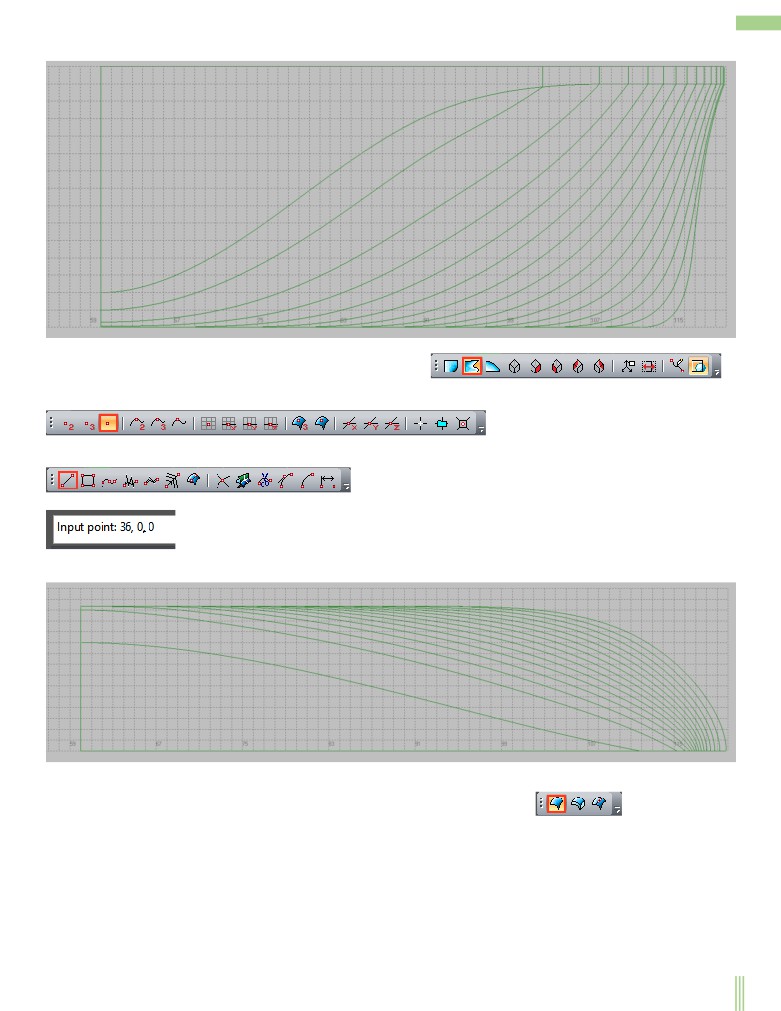
Specifies the spatial lines.
There are several ways to define lines. We will only consider the most commonly used.
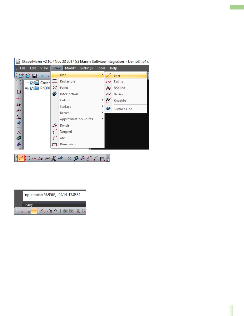
You can start entering lines by using the following command.
or by pressing the button from the Toolbar Create:
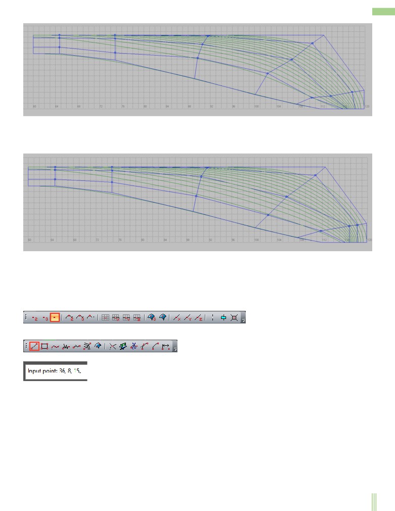
The spatial lines are specified by the start and end point. A straight line is held between the points. Point coordinates can be specified
as the cursor in the work window, and with the use of object and topology bindings. If necessary, precise coordinate values can be
specified by the keyboard.
After you select a command in the coordinate entry line you receive the following message
and the coordinates of the current point are displayed. Clicking Enter You can use these coordinates. If you need to enter other
coordinates, just click the cursor in the coordinate input field or the left or right arrow on the keyboard and edit the line with
coordinates. After entering the first point of the line, the system memorizes the coordinates of the entered point as the coordinates of
the current point and gives a message for the next point. The rubber thread from the first entered point to the cursor location appears
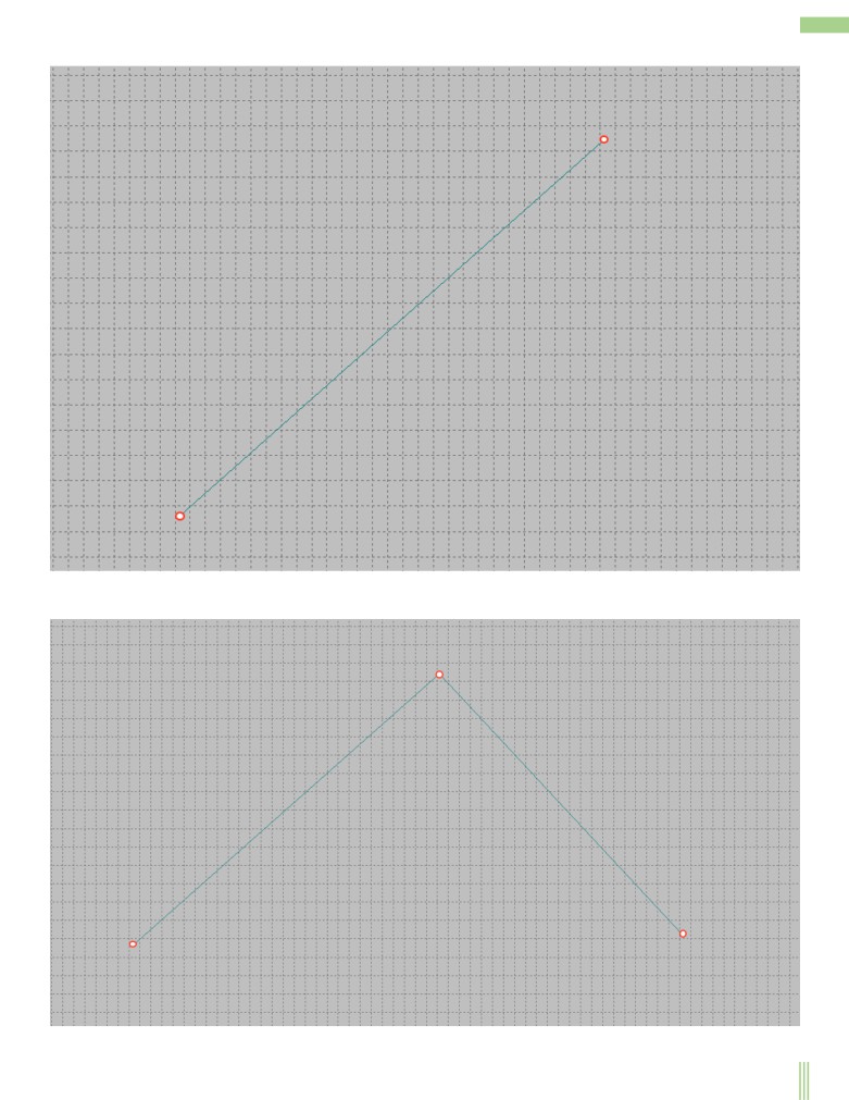
44
on the screen. After entering the second point, a straight line appears on the screen.
The line is drawn in the current color and is written to the current block. The entered points are also written to the current block. After
you enter the second point and the line appears on the screen, you can continue typing the next point. This will show the 2nd line
having a common point with the first line.
45
In this case, the entered lines topologically connected to each other through a common point. That is, when you change the position of
a shared point, both lines are changed. If you do not want to enter a chain of related lines, you can click Esc or right-click and start
entering the first point of the new line. When you enter new lines, you can change the projections, the work plane, and the work
volume.
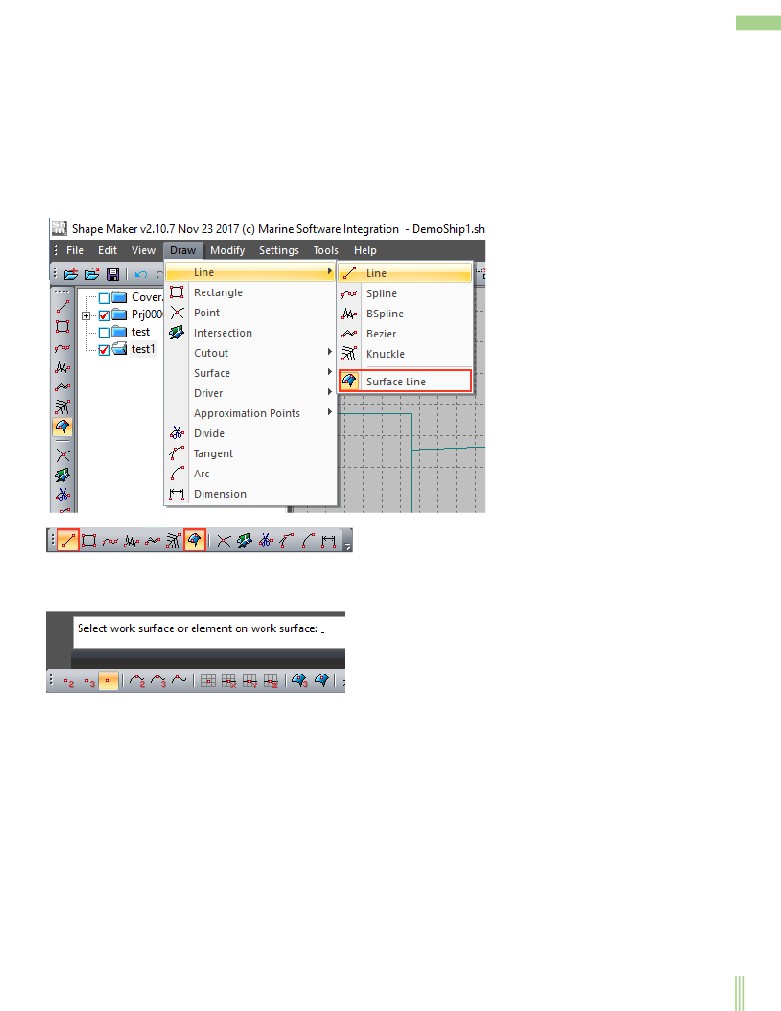
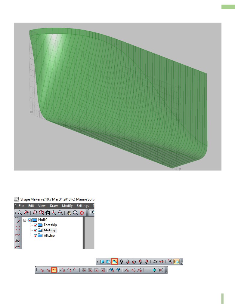
Specifies the surface lines.
The lines on the surface differ from the spatial lines in that the shape of the line is defined as the intersection of the projection line
with the surface on which the line lies.
You can start entering lines on the surface with the same command, with one difference - the surface line input mode must be
enabled.
or by pressing the button from the Toolbar Create:
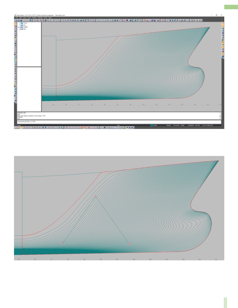
The system uses the concept of the current surface to enter surface lines. When you enter the first surface line since the start of the
session, the current surface is indefinite, so the following message is displayed in the Coordinate input window.
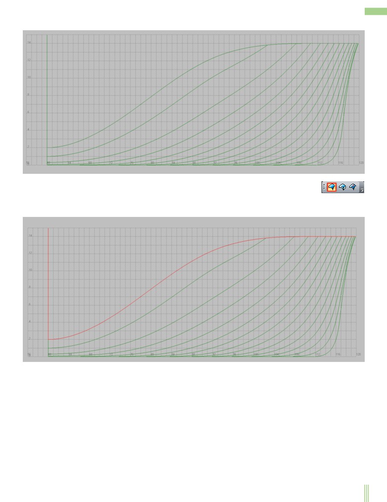
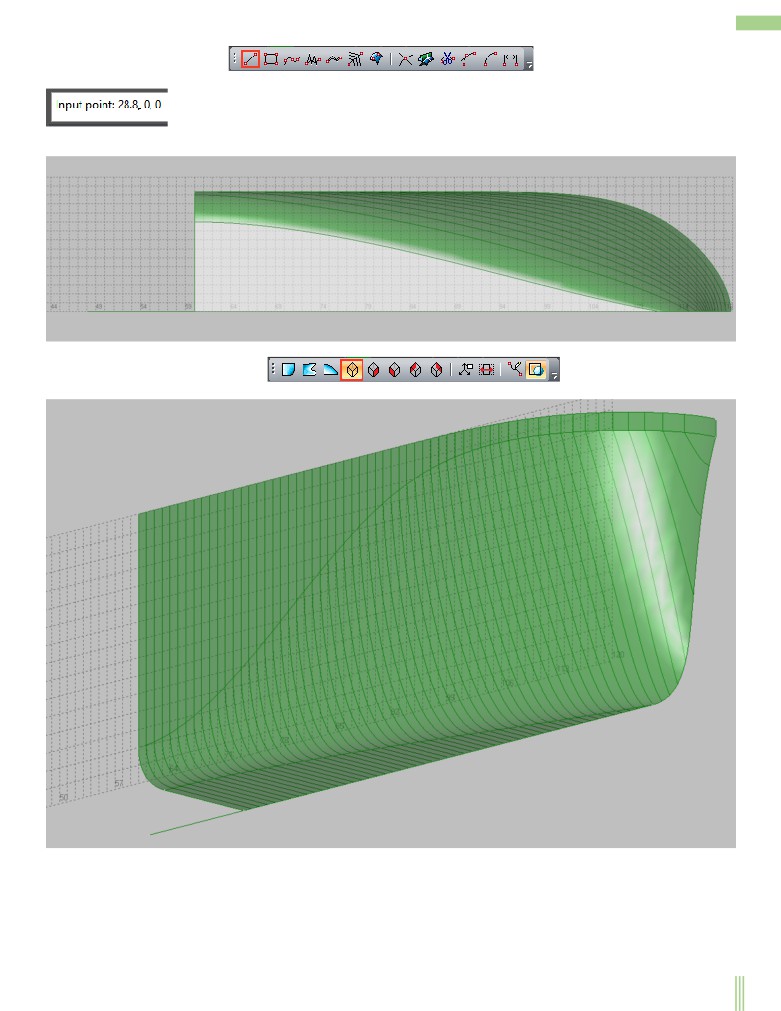
Specify the current surface to enter surface lines you can click on this surface in the work window or enter the name of this surface in
the coordinate input window.
46
The contour of the selected surface is highlighted red. If you enter all subsequent surface lines per session, the current surface contour
will always be highlighted red. The input of surface lines is carried out as well as the spatial lines, but with some limitations:
-Surface lines must be entirely within the boundaries of the surface or be topologically connected boundary points with surface
boundaries.
-The surface area on which the surface lines are set must be unambiguously defined on this projection.
-The line should not intersect the contour of the surface.
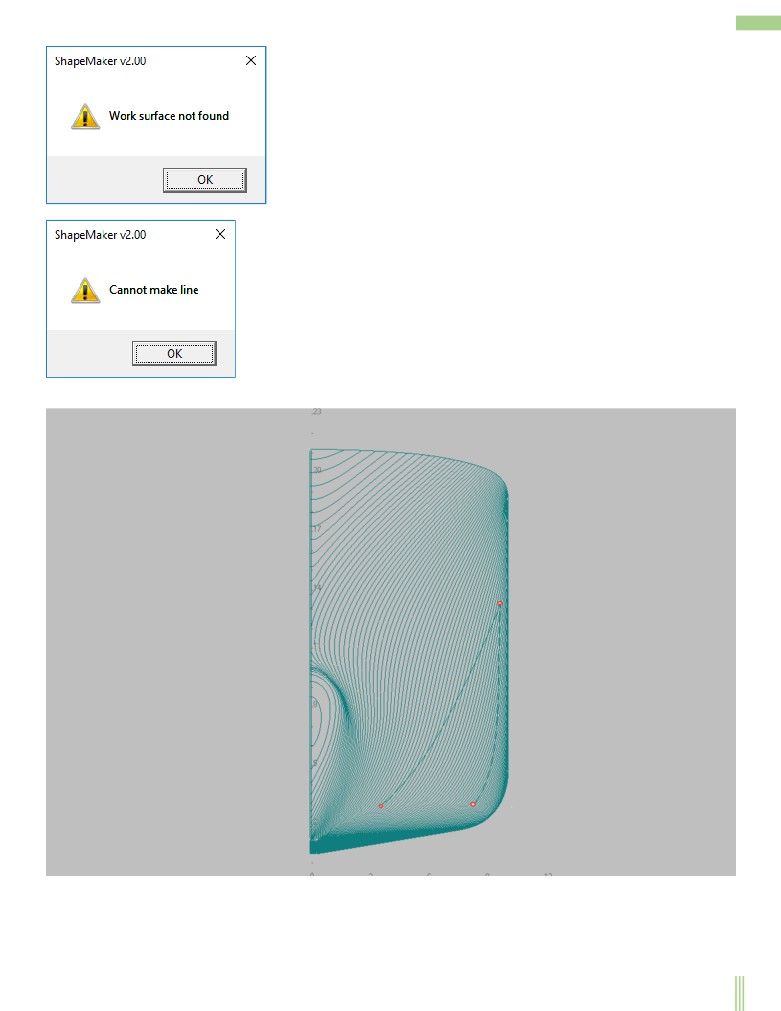
If you enter one of the points outside the surface contour, the following message is issued:
47
If for any of the above reasons you cannot build a line, a message is issued.
As a result of the successful construction of the line on the projection with which the line was set this line will look straight.
When you switch to a different projection, you can see that the lines are projected onto the surface.
48
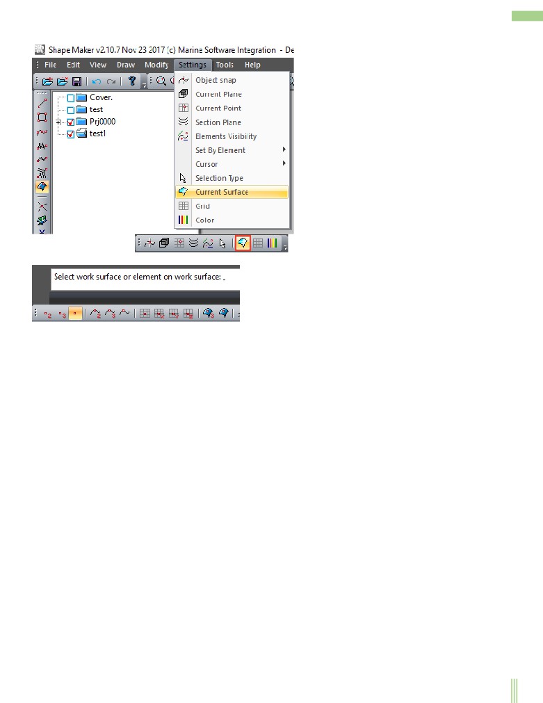
If you need to change the current surface while entering surface lines, you can do this by following the command.
or from the toolbar Settings:
A question will appear in the coordinate input line:
You can specify a new work surface without interrupting the input of surface lines.
A surface line cannot be built simultaneously on multiple surfaces. On each such surface of a line it is necessary to define separately.
Only boundary lines and corner points of the current surface and lines and points lying on this surface can be used as Object snap
objects when entering a surface line.
49
Changes the shape of the spatial lines.
To change the position of line endpoints
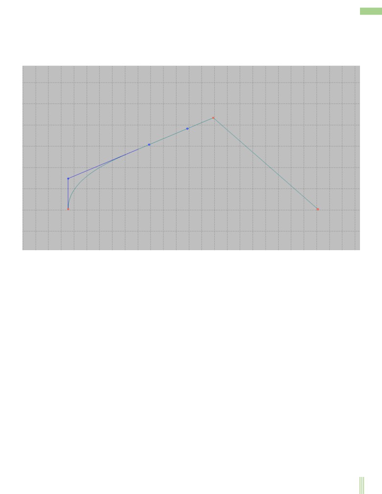
By default, all input lines are straight. The simplest way to modify a line is to change the position of its endpoints. Since the system is
always in edit mode, it is enough to click the left mouse button on the editable point and move it to a new position and by clicking
once again to fix the point in the new position, as shown below.
In this case, the point you are editing converges on two topologically linked lines. Therefore, both lines followed the point when its
coordinates changed.
Edits the shape of the curve.
It is often necessary to change the shape and line not only the position of its endpoints. To do this, click the left mouse button on the
line whose shape you want to change.
The system will show the control polygon for this line.
50
Changing the shape of the control polygon will dynamically change the shape of the editable line. By default, the control polygon has
two control points. The direction of the vector from the end point to the intermediate point of the polygon shows the angle of the
curve of the end point, and the length of the vector indicates the degree of line fit to this vector at the end point. So if the vector is
positioned horizontally or vertically, we will have a horizontal or vertical tangent at that point. By editing the points of the control
polygon, you can try to achieve the desired shape of the curve.
Changes the number of control polygon points.
Ship curves are often more complex than the curve shown above. More degrees of freedom are required to describe these curves. In
our case, more checkpoints are required.
There are several ways to add additional points to a control polygon. The easiest way is to click the left mouse button With pressed
simultaneously Ctrl To the line connecting the control points to each other. The system adds an additional control point to the control
polygon. The shape of the curve will not change. If you want to reduce the number of points you need to right click, pressing
simultaneously CtrlOn the line between control points. This method allows you to add a certain number of control points from the
next row: 4, 5, 7, 11, 19, 35, 67. The reasons for using such a series will be explained later.
51
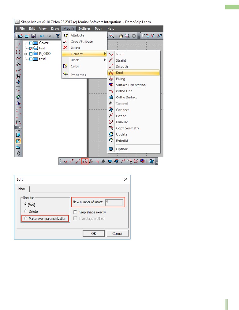
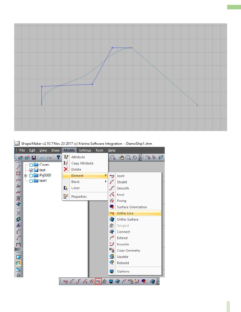
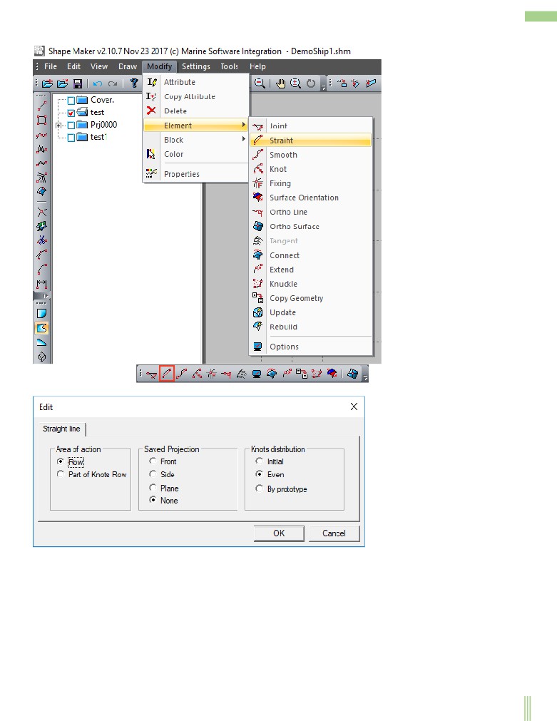
You can also add and remove an arbitrary number of control points by using the following command.
or from the toolbar Modify:
In the dialog box, use the marked options to set the number of control points you want.
52
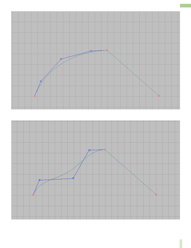
An additional control point will make it more possible to change the shape of the curve. Now we can change the shape of the curve
keeping the angles of inclination of the start and end point.
Specifies the tangents at the end points of the curve.
It is often necessary to set tangents at the start and end points of a line strictly horizontally or vertically. To do this, just click the left
mouse button with the button Ctrl To the line between the end point and the first control point of the polygon. In this case, the tangent
53
will be displayed horizontally or vertically, depending on the initial tangent angle at that point. If the inclination angle is less than 45 °
tangent will be horizontal, if more-vertical.
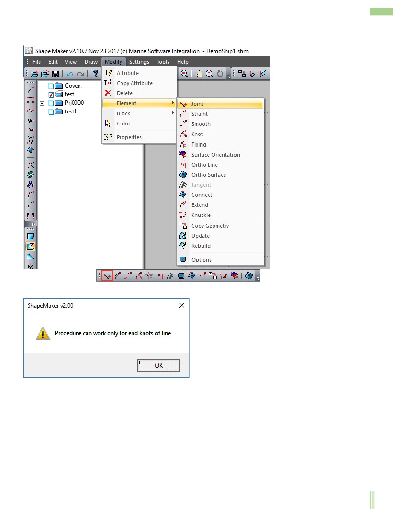
The same can be done by calling the appropriate command from the menu.
or from the toolbar Modify:
54
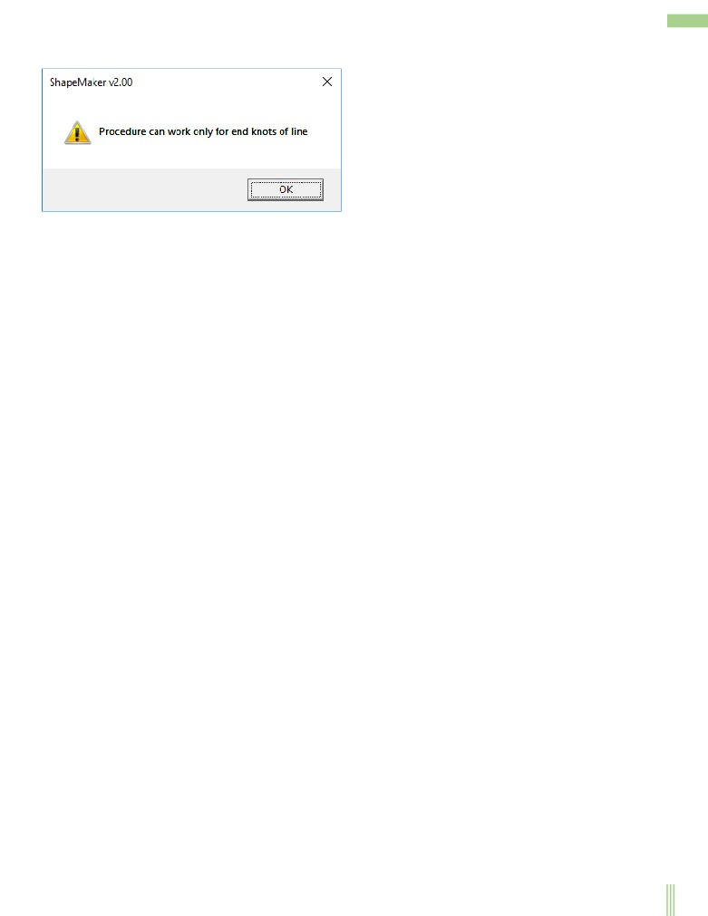
Note that in this case the dialogue is organized somewhat specific. Before you call this command, you must have the last point that the
user edited was one of the points of the closest endpoint of the line. Otherwise, the following message appears.
Simply put, the system should be made to understand which of the tangents should be placed horizontally or vertically.
55
Fillet curves.
There is often another task when you want to make smooth connection of this curve with another that has a common point. The user
must first approximate the tangent angle at that point and then call the next command.
or from the toolbar Modify:
Before you call this command, you must have the last point that the user edited was one of the points of the closest endpoint of the
line. Otherwise, the following message appears.
56
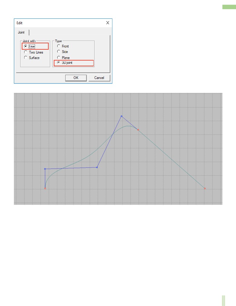
If the editable point is selected correctly, in the dialog box that appears, select the specified functions and click Ok.
The tangent to the line will be displayed accurately.
The system allows to seam curves both in space, and on one projections. It is also possible to dock with the surface and with a plane
formed by two lines.
57
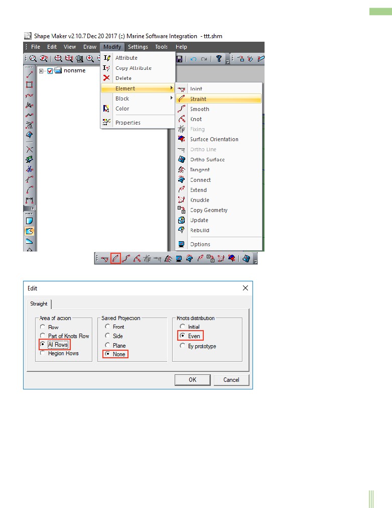
Straightening lines.
One of the advantages of this type of curves is the ability to flatness the entire curve or part of the curve. For this purpose, it is
necessary to put a number of control points on one direct. The easiest way to do this is by clicking the left mouse button with the
button Ctrl To the starting and ending points of the area of the control polygon to reroute. In this case, all the intermediate points of
the selected area will be projected to the straight, formed by the start and end point. The projection type will be determined by the
angle of this straight to the horizon. If the angle is less than 45 °, the points will be projected vertically, if more-horizontally.
58
The advanced option of flatness curves can be used to call the following command from the menu.
or from the toolbar Modify:
The flatness curve dialog describes almost every possible case.
59
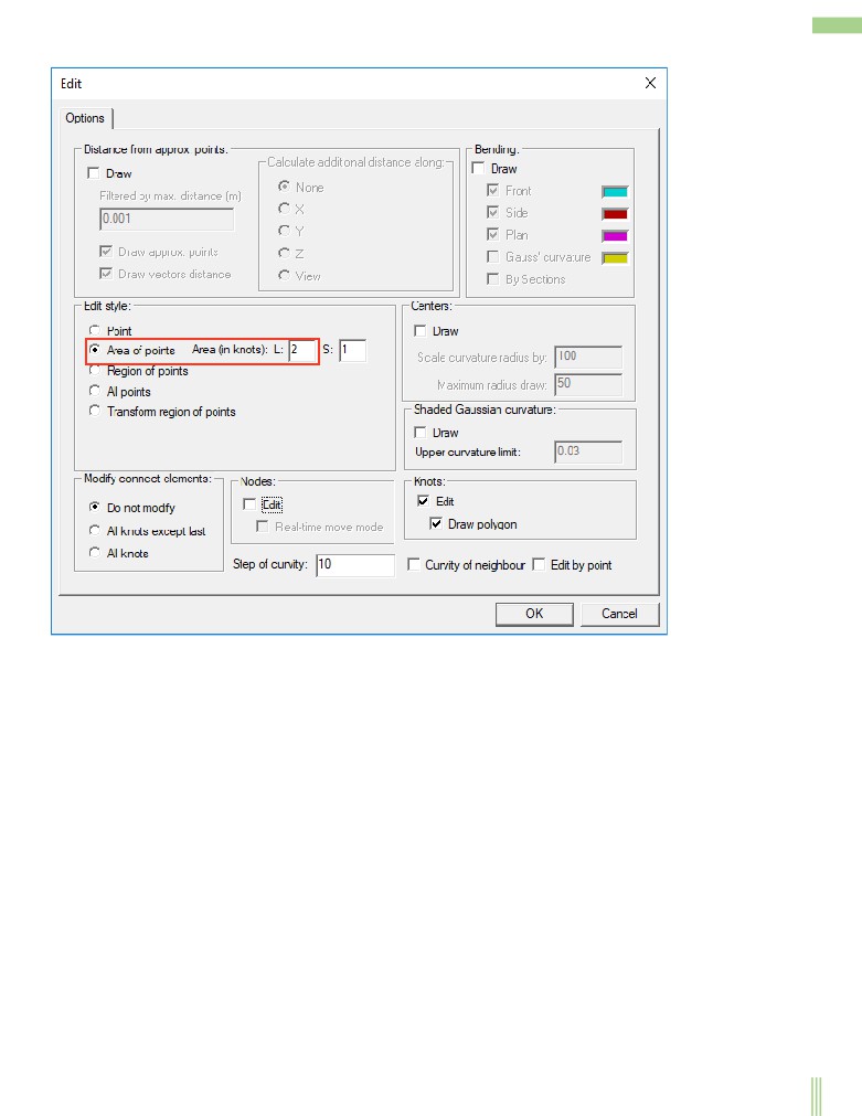
Edits the Polygon Control Point group.
Sometimes there is a need to change multiple control points at the same time. For this purpose the mode of modification of a group of
control points of a polygon is intended. By default, a single control point change mode is in effect. To switch to the control point
group Editing mode, click the left mouse button next to the Bar status window.
Then set the number of points to change in the next field status bar.
If you click the left mouse button The number of points will increase, and if the right-to decrease.
Modification of the group of control points shown above is performed at the following values.
As you can see in the image, the center point is moved by the cursor, two points on the left and right are followed by the center point
being moved. For convenience, the control polygon, which is changed when the center point is moved, is highlighted with yellow
lines.
60
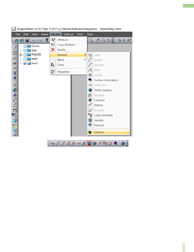
Enabling this mode can also be done by the following command.
or from the toolbar Modify:
61
and selecting the marked mode in the dialog box that appears.
62
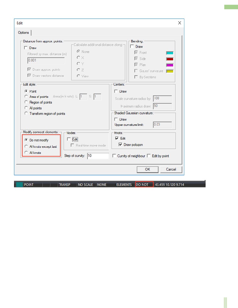
Modes of changing the shape of the curve when the position of its end point changes.
Because the objects in the system have topological relationships and are dependent on each other, when you change the position of the
control point, the curve must change its shape.The system has three different Mode Variationя Shape of the curve when the position of
its final intersи. You can set one of these modes by using the command.
or from the toolbar Modify:
63
and select one of the three possible options in the dialog box that appears.
The same can be done by left-clicking in the Next Status bar field.
One of the modification modes is always current. Consider how these modes affect the shape of the line.
64
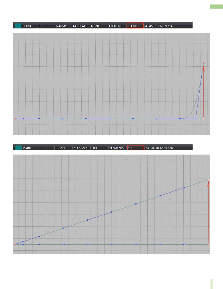
1.
Mode without modification of points controlOn Curve polygon.
In this mode, when the end point position is changed, all points in the curve control polygon remain in place.
This mode is used when you want to save the shape of the curve and only modify its end point.
-Mode of modification of all control points of the curve.
In this mode, changing the position of the control point will change all points of the control polygon by linear rule.
This mode is useful when you want to change the entire curve without paying attention to the tangents in the endpoints.
65
- The mode of modification of all control points of the curve except for the control points nearest to the endpoints.
In this mode, the tangents are not changed at the start and end point. All other intermediate points are recalculated by linear rule. This
mode is useful if you want to preserve the tangent curve value of the endpoints. For example, to maintain a smooth fillet of two
curves in the editable point.
The last two modes can work in conjunction with the modification mode of the curve control points.
In this case, only the part of the curve that is specified in the modification mode of the curve area is modified.
66
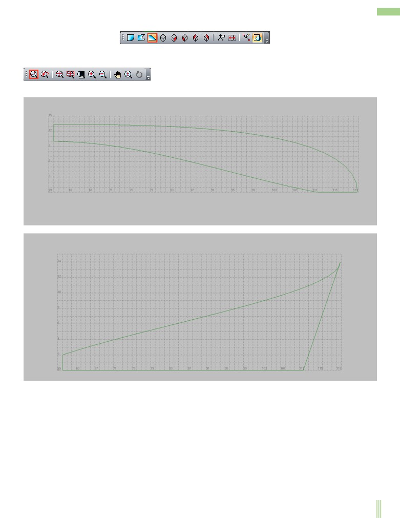
Smoothing Form Curve.
Smoothing is a very important process on which the surface quality of the hull depends. The means of visual quality control of the
curve play an important role. The properties of B-spline curves give us significant advantages of such control.
Let's point again on the properties of B-spline curves. As mentioned above in the form of a control polygon we can define the angles
of the curve input at the endpoints. If the polygon is convex, the curve has no inflections. If more than three points of the control
polygon lie on one straight curve will have a straight section. All these properties allow you to control the shape of the curve
according to its polygon shape.
In addition, the system provides visualization of the radius of curvature of the curve and inflection points. Compression of the curve
image on one of the coordinate axes is also a good control tool. In fact, this is analogous to how the designer controls the shape of the
line looking along the curve, almost in the drawing plane. This function is especially useful when it is necessary to simulate curves
elongated in one direction, such as the profile of the wing of the plane.
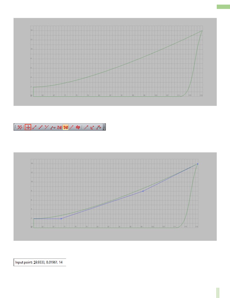
The essence of the smoothing process is to obtain a smooth curve as close to the given prototype as possible and aesthetically
satisfying our view of it. This is a very subjective process. Two people can draw completely different curves. Therefore, the ideal
smoothing process is a combination of manual and automatic mode.
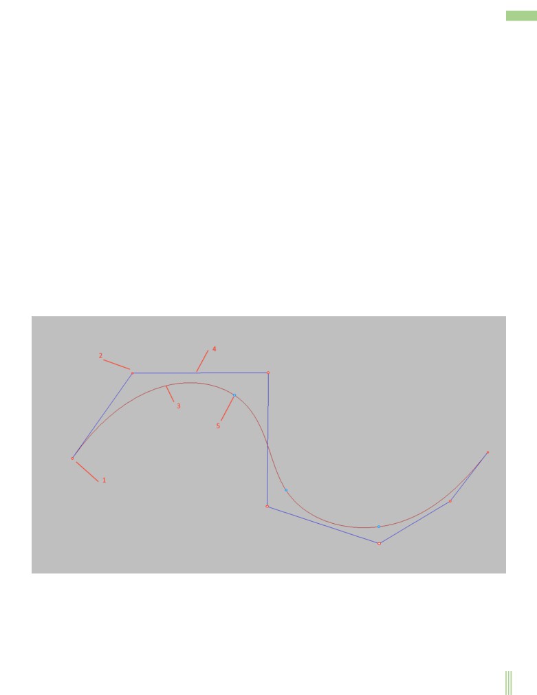
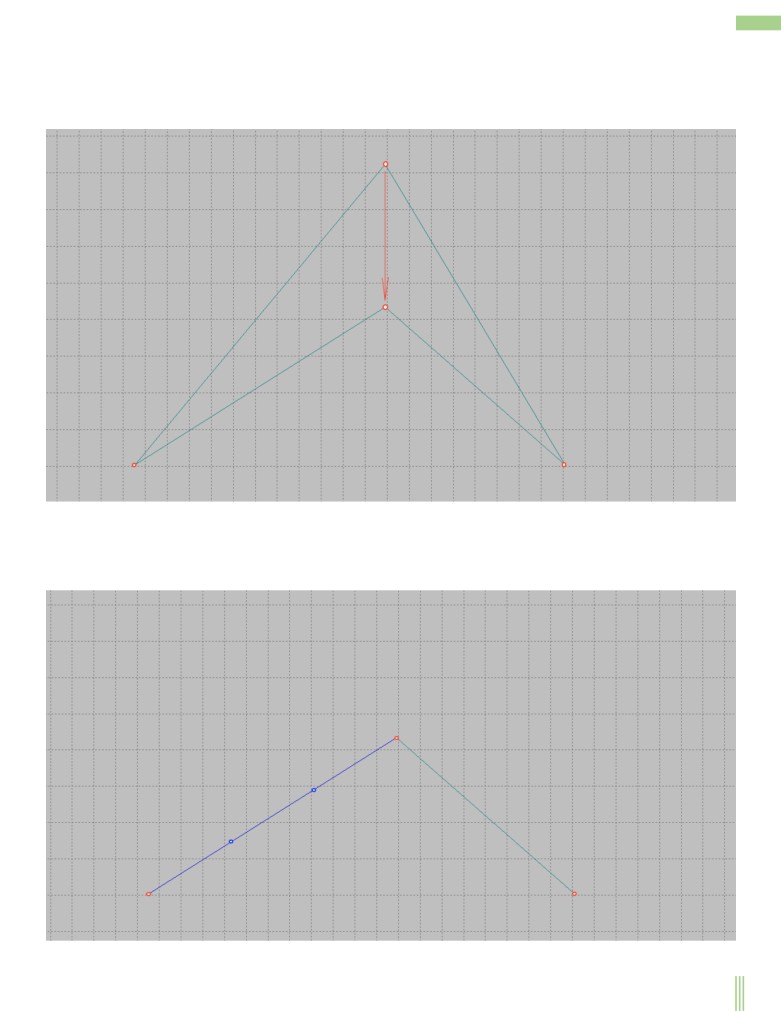
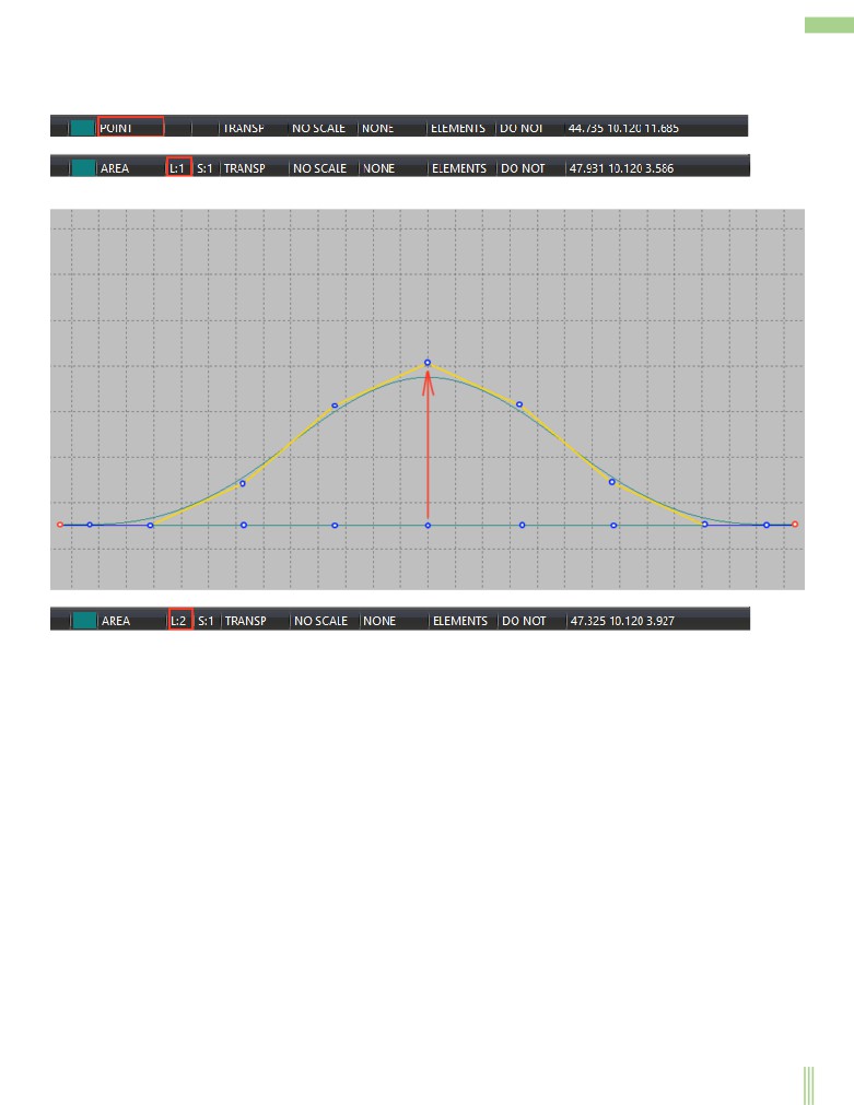
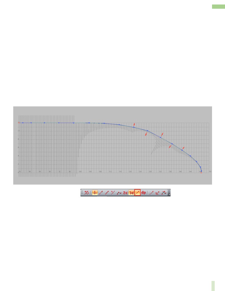
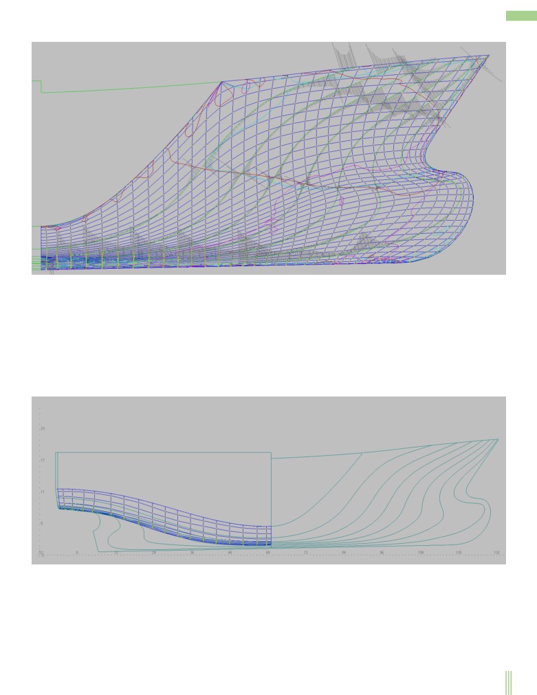
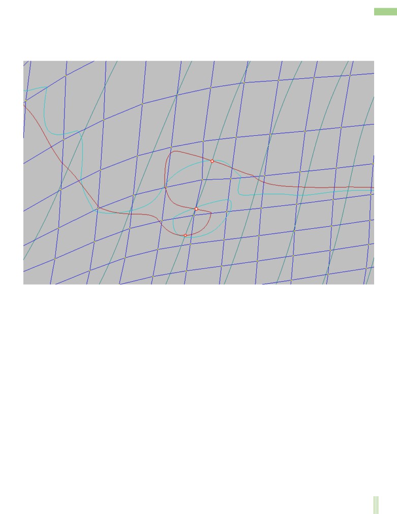
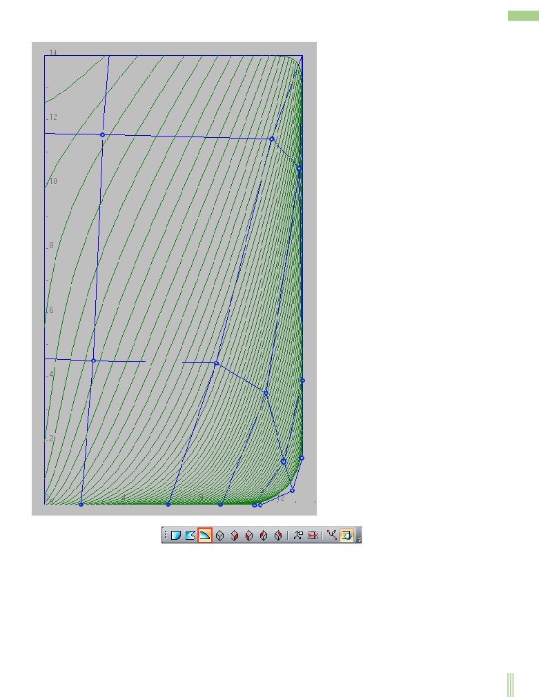
Example of smoothing the deck line. The curvature radius graph shows the areas of the curve that require correction. The biggest
mistake of beginners is to try to smooth out the curve by moving only one point. The Red Arrows show how to change the position of
several control points to achieve a good result. When you change the position of the control point, the curve shape and the curvature
radius graph are automatically changed. As a rule, only a small movement of control points is enough to significantly change the
curvature chart.
Therefore, to move the points of the control polygon when smoothing use the scaled cursor movement. Recall that this mode is set by
pressing the following toolbar button Marker.
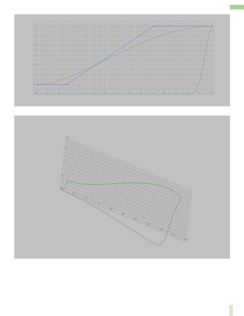
67
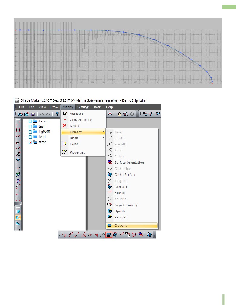
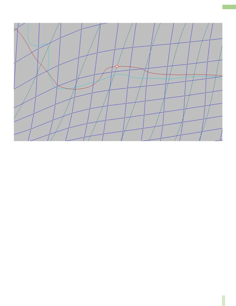
As a result of smoothing points it is easy to achieve such result.
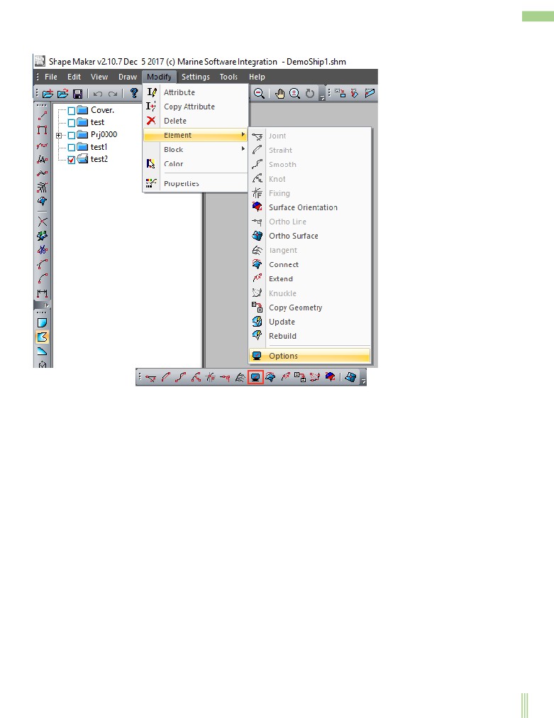
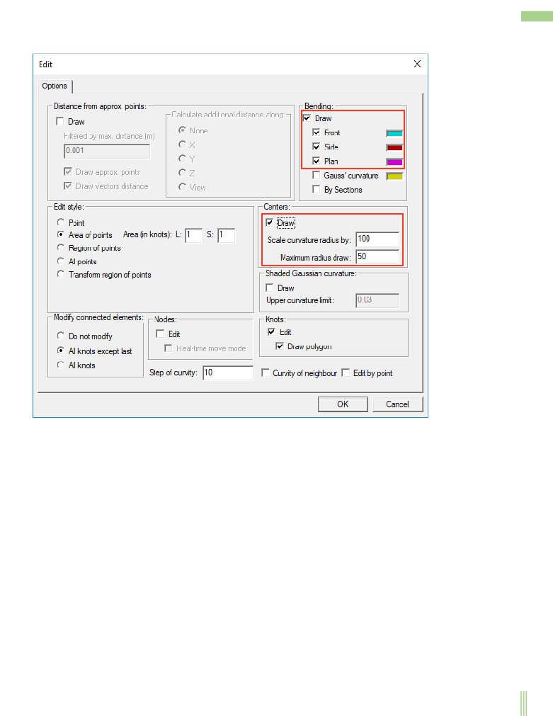
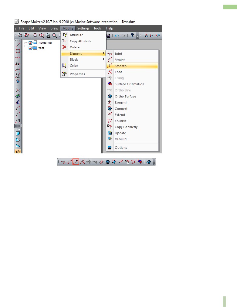
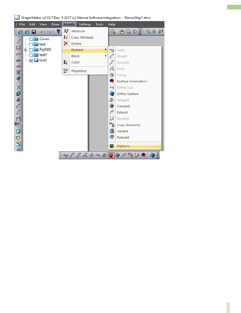
You can show a chart of curvature radii using the following command:
or from the toolbar Modify:
68
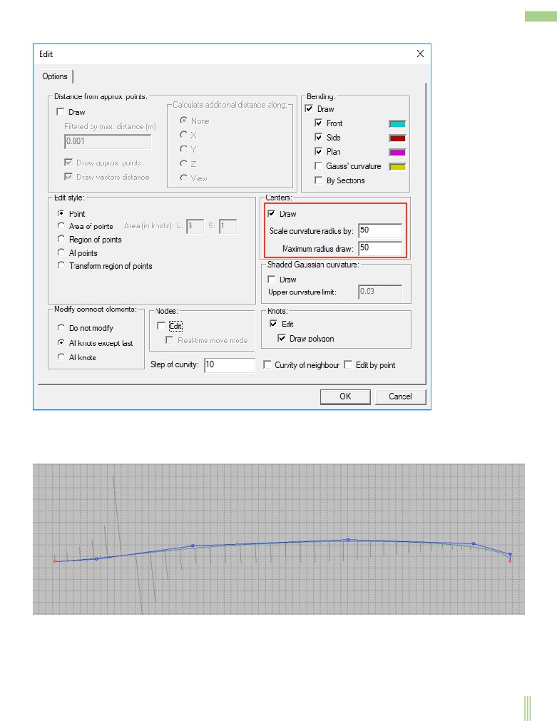
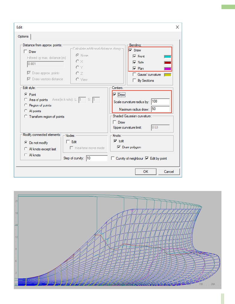
and setting the specified fields in the next dialog.
For ease of visualization, the curvature radius chart is scaled to the corresponding scale factor. To avoid a large number of lines on the
screen, the radiuses of curvature are trimmed more than the specified value.
As mentioned earlier for the design of large extension lines, such as profile the airplane wing is used to compress the screen by length.
The line shown below has a large elongation. The form of such a line is difficult to control.
69
If you use the screen compression along the length, the line will look like this.
It is important to note that only the image on the screen is compressed. All the coordinates of the control points remain on the real
scale. Editing such a curve is much simpler.
And if the curve looks good in a compressed form, it will only look better in real scale.
70
Recall that you can switch to the visualization mode of the compressed screen by clicking on the next field in the status bar.
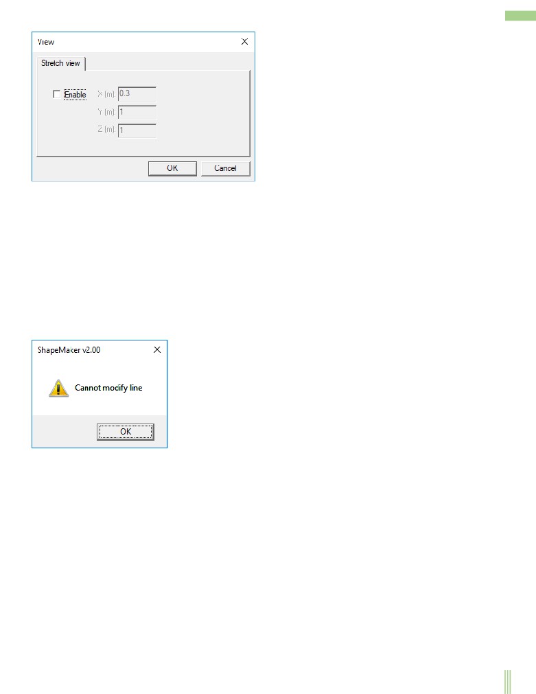
You can set the compression ratios on the coordinate axes by the following command.
or from the toolbar View.
and set the compression ratios by coordinates axes n the following dialog box.
71
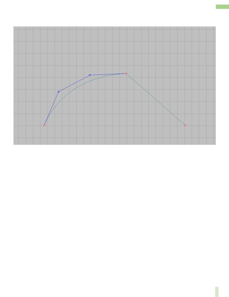
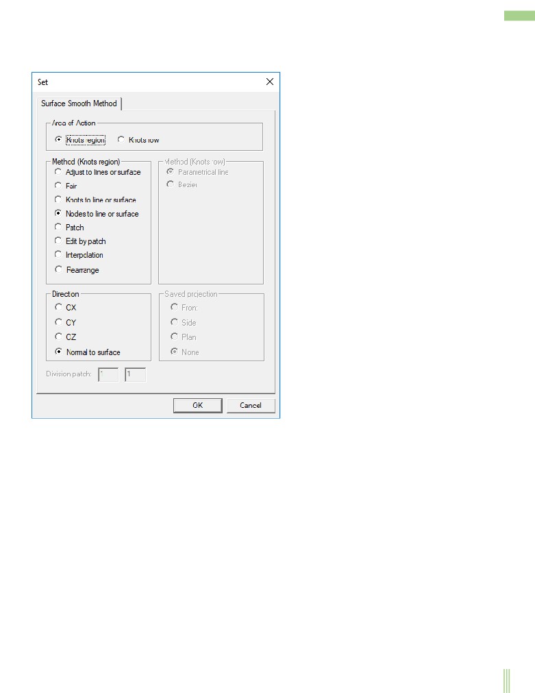
Smoothing the curve is a very subjective process. Therefore, this section focuses on the smoothing of the curve manually. The system
has several different methods for automatically smoothing curves. In this section we recommend only one of them. To smooth out a
part of a curve it is enough to click on one of control points with the control key pressed, then to specify the second control point. The
specified control point area will be modified to achieve the desired smoothness of the curve in the area. If the smoothing result does
not satisfy, you can repeat the procedure.
Changes the shape of the lines that lie on the surface.
All that has been said above about the editing of spatial lines fully refers to the lines lying on the surface. When editing a line lying on
a surface, remember that it is possible to edit only the projection from which the line was defined and only on this projection the shape
of the line will correspond to the shape of the control polygon. Other projections of this line are calculated as the result of projecting
to the surface.
If you cannot project the line correctly when you edit the surface line, a message appears on the surface.
72
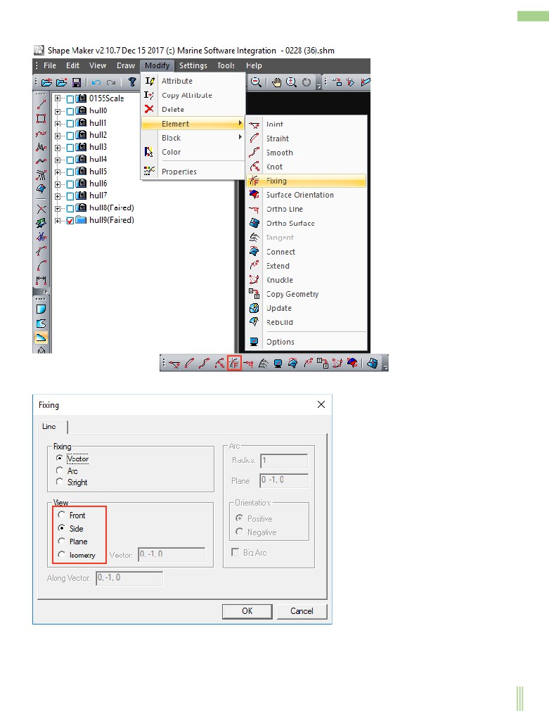
Note that in the editing process you can change the projection of the line. You can use the menu command to do this.
or button from the toolbar Modify:
and select the appropriate projection in the dialog box.
73
Working with surfaces.
To specify a surface shape, the program uses a third-degree B-spline surface. From a mathematical point of view this means that
within a single area of the surface smoothness is performed on the first derivative (angle of inclination of the tangent at the point) and
the continuity of the second derivative (curvature at the point). The third-degree surfaces are best suited to describe the shape of the
ship hull. Such surfaces allow to achieve the required smoothness and, at the same time, locality of changes.
The feature of these surfaces is also that the connection of two patches of the surface can be done only by the first derivative (angle of
inclination). This is perfectly permissible when the fore ship surface is connected to a cylindrical midbody, a flat side, or a flat
bottom. In case of joining of two curved patches of a surface between itself the form of a surface in a place of a connection has an
aesthetical kind. Very often such a surface is quite difficult to fix. Therefore, it is recommended to use one curved surface on the fore
or aft ship if possible.
The most part of work on change of a surface form is necessary for change of position of points of control polyhedron. The correct
location of the control polyhedron grid is very important for getting the correct surface smoothing result. Equally important is the
uniform distribution of the parameter on the surface grid.
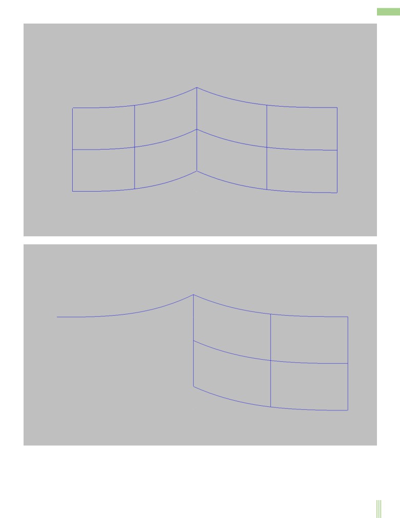
The surfaces definition.
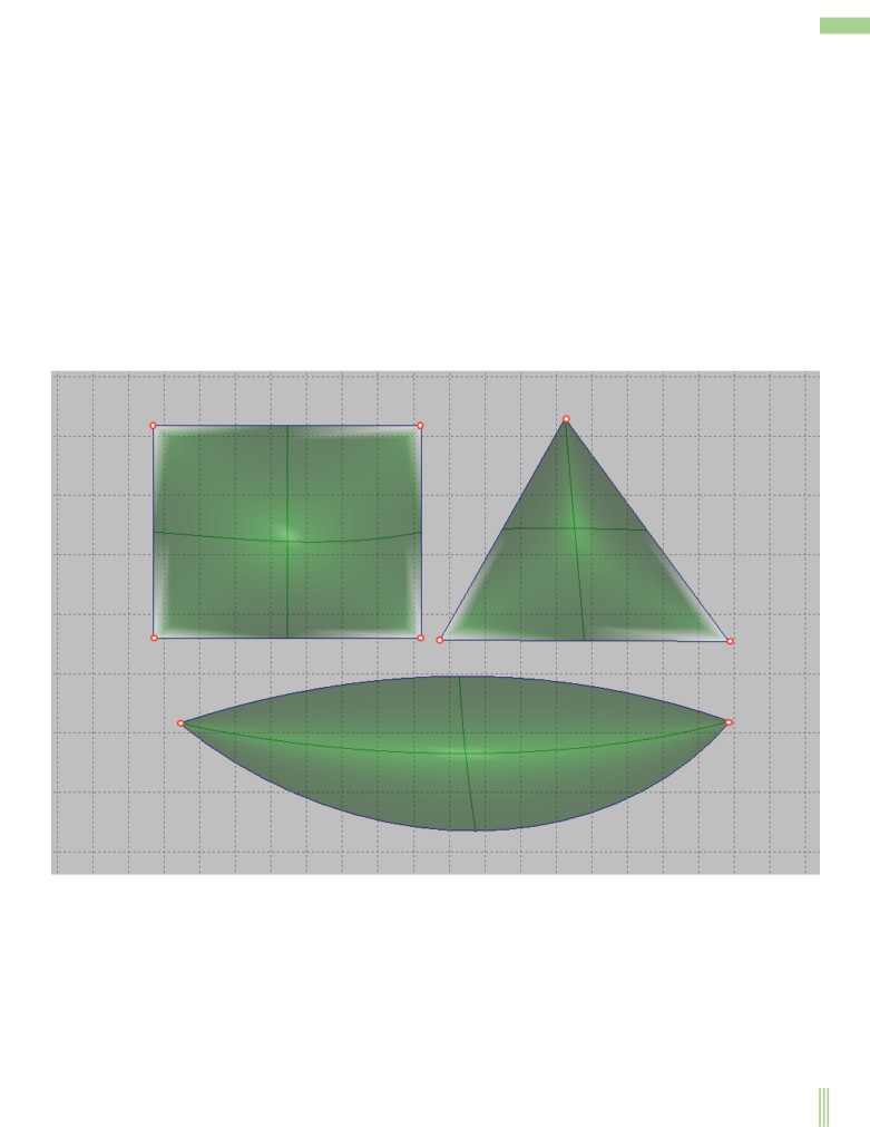
Due to the mathematical peculiarities of the-spline surface, the system supports surface patches formed by four, three and two
boundary lines.
In fact, the case with three and two boundary lines is a private case of a plot with four boundary lines, where part of the boundaries are
degenerate into points.
74
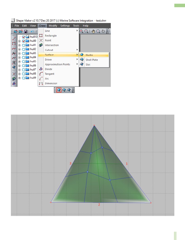
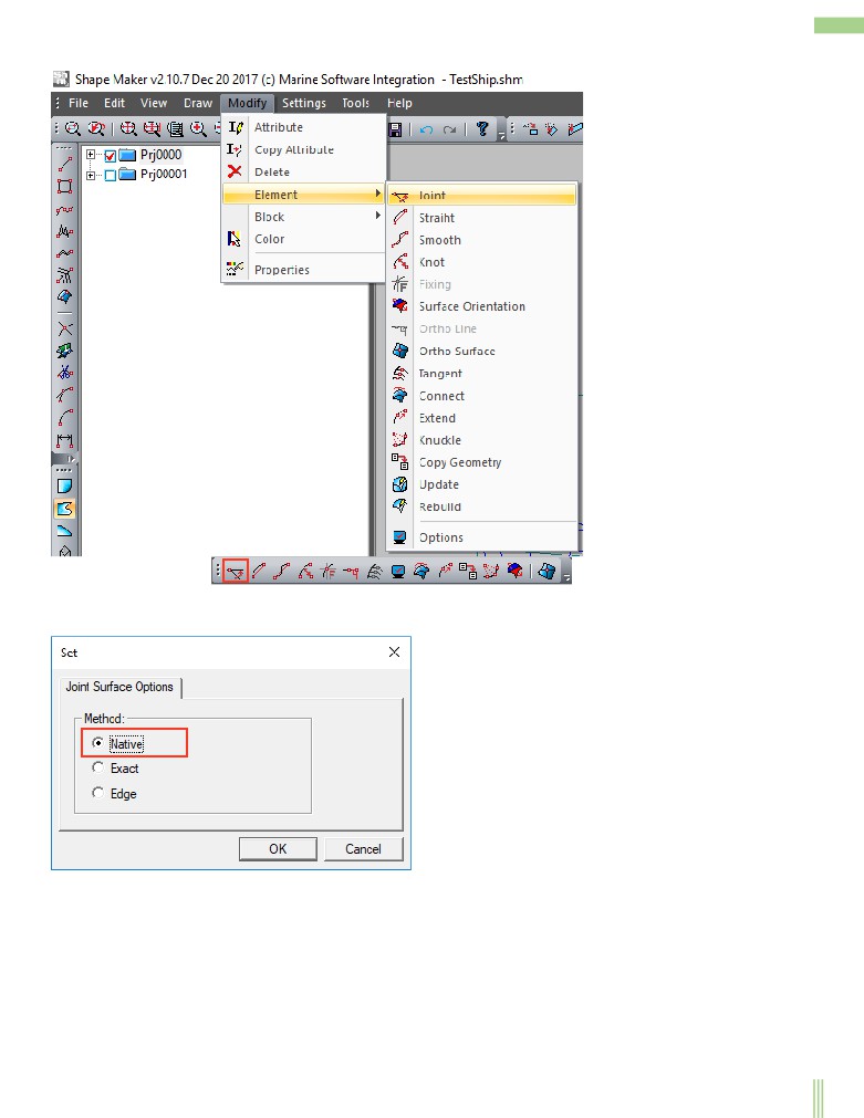
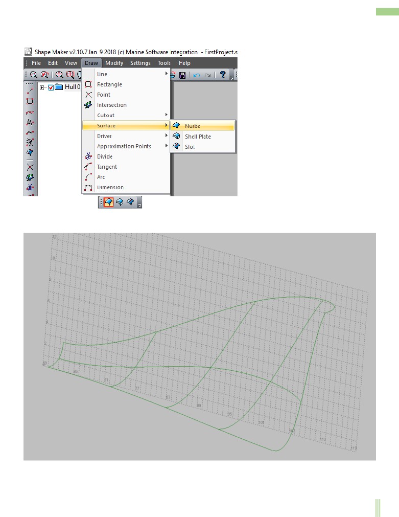
You can use the menu command to specify the surface.
or button from the toolbar Surface:
Then set the contour of the chain line and click Enter. During selection, the marked lines will be highlighted red. Each subsequent line
will be selected as a contour line only if it has a topological relationship with the previous one.
When specifying a surface patch with three boundary lines, it is important to understand which of the boundaries will be degenerated.
There is a simple rule - the first point of the first marked line will be the degenerate boundary of the triangular area of the surface. The
sequence of setting the parcel boundaries is shown in the following figure.
The position of the degenerate surface boundary strongly affects the properties of the triangular surface and the location of the control
polyhedron points.
75
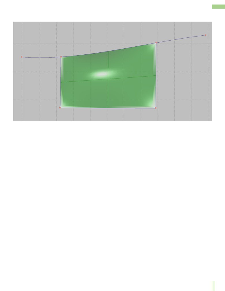
As shown in the figure below, a part of a line can be used as the boundary of a surface topologically connected to other contour line
through a hinged point.
Controls the number of surface control points.
Number of surface control points in the system Shape Maker not specified by the user, but generated by the system itself, depending
on the number of points on the boundary curves of the surface. Although the user can specify any number of control points at the
borders, it is better to follow a specific rule. To understand this, let's look at how the system calculates how many control points
should be inside the surface.
The system uses third-degree lines and surfaces. This means that the number of intervals of elementary Beziers of curves of the third
degree inside В-spline is calculated by the formula:
Number of intervals = number of control points-3.
In this case the minimum number of control points of the curve is 4. The endpoints coincide with the beginning and end of the curve.
The other two intermediate points specify the tangent direction and the degree of adjoining to the tangent at the corresponding
endpoints.
If the curve has four control points, it is simply a Bezier curve with one interval.
If the control points are five - two intervals and so on. Interval boundary points are called curve nodes.
When you specify a surface, the condition of mathematically exact match with the boundary curve is observed. The number of nodes
on the surface is computed as superposition nodes of opposite surface boundaries. If the number of nodes at the boundary is the same,
in this case the surface will have the same number of nodes and correspondingly the same number of control points.
76
The resulting surface, built on the upper border with five control points and the lower border with four, is shown below.
According to the above formula, the five control points give us two intervals on the curve connecting to the node. The curve parameter
will accept the following values:
- At the start point of the curve,
- In a node
- At the end point of the curve.
The lower curve has four control points, one interval and has no intermediate nodes. When you build a surface on such boundaries, the
Shape Maker automatically creates a node on the lower edge that corresponds to the node parameter at the correct boundary. In our
case, the node parameter value will be-0.5.
The values of the nodes are based on the surface. In our case in the longitudinal direction on a surface there will be five control points
two intervals of a surface representing an elementary surface of Beziers of the third degree. A line that intersects a surface in a vertical
direction is just a line of division into Bezier areas or a line of equal parameter with a value of 1.0.
Summing up the surface creation algorithm creates nodes on the curve that correspond to nodes on the opposite curve. The surface is
created on curves that contain all these nodes with the adjacent curves. If the node settings on the adjacent curves do not match the
new nodes, the number of control points on the surface does not increase. Ideally, the number of control points on the surface must
match the largest number of points on one of the curves. Such conditions create some inconvenience for the user but have one very
important advantage-in this approach to the creation of surfaces the total boundary of the two surfaces is mathematically accurate.
That is, there is no gaps between the surfaces.
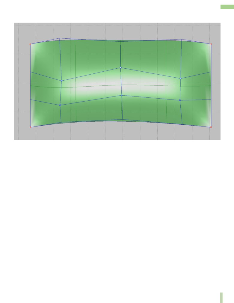
If the number of nodes does not match, all nodes corresponding to each boundary are added to the surface. This circumstance can
dramatically increase the number of control points on the surface and make editing such a surface very difficult. Another very
important circumstance-the dissimilar nodes on the surface can be added very close to each other in the parametric space of the
surface. The properties of surface control points with uneven distribution of nodes are very different from uniform distribution and
interfere with smoothing surfaces. This circumstance significantly interferes with the modelling of surfaces. Below is an example of a
surface where the upper bound has 6 control points and the bottom 5. The resulting surface has 7 control points.
77
The above problems are easily avoided if you use combination of control point numbers when specifying boundary lines, where nodes
with uniform distribution of the parameter will be added to the surface. The set of control points “magic” numbers is a series: 4 5 7 11
19 35 67... According to the formula, the corresponding number of intervals will be 1 2 4 8 16 32 64
Accordingly, nodes on
opposite boundary curves will be either coincident or located in the middle of the interval between neighboring nodes. If you use
numbers of this series to specify boundary lines, the resulting surface will always have a uniform distribution of the parameter. In this
case, the number of surface points will match the maximum number of points on the boundary curve. This circumstance allows to
specify different number of points on neighboring surfaces. For example, a stem line can have 35 control points. The opposite line of
bulge radius at the entrance to the parallel midbody has only 5 points and the resulting number of points on the fore ship surface will
be 35. In this case, the cylindrical surface of the bulge radius will have only 5 points. A stern surface connected to a parallel midbody
can have, for example, 19 points if there are 19 control points on the transom line. It is worth noting that the observance of “magic”
numbers is not a large limitation in the system and is important only for complex curved surfaces. If the surface is flat or cylindrical,
the number of points can be any. If one of the edges of the surface is drawn on a part of a line-it is recommended to lead a hinged
point strictly in a knot of a curve and to calculate number of control points on the opposite boundary based on number of knots on a
part of a curve. This will also give a uniform distribution of the nodes on the surface.
The number of control points on the surface changes when the number of checkpoints on the boundary curves changes. The position
of the new control points is selected from the maximum retention condition of the surface shape. This allows increase the number of
points in the surface shape editing process when the existing number of points is not sufficient.
Surface visualization.
The visual representation of the surface shape is very important for the smoothing process. The system provides several different
visualization options for surfaces.
78
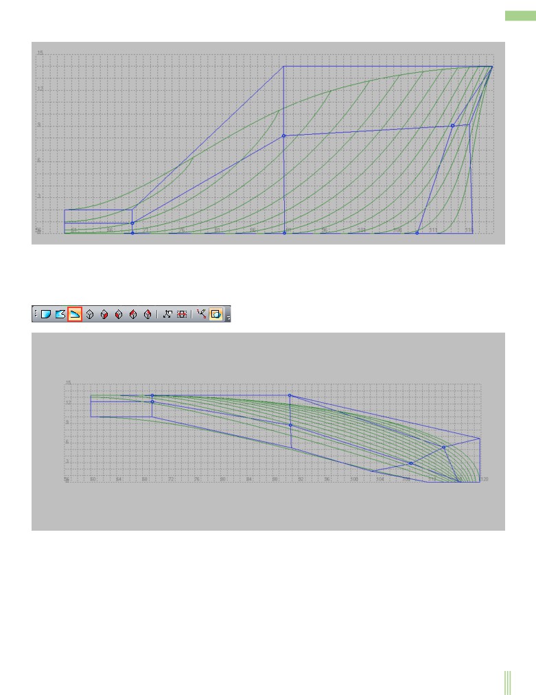
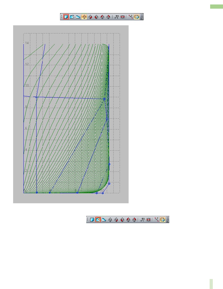
Line of an equal surface parameter.
These are curves that have a constant value of one of the parameters in the parametric representation of the surface. Lines of equal
parameter give an idea of how much evenly distributed points of the control polyhedron surface. The line shape of an equal parameter
is automatically recalculated when the position of the control polyhedron points changes.
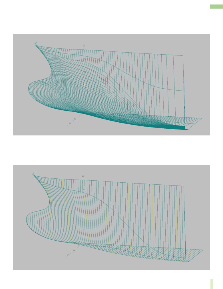
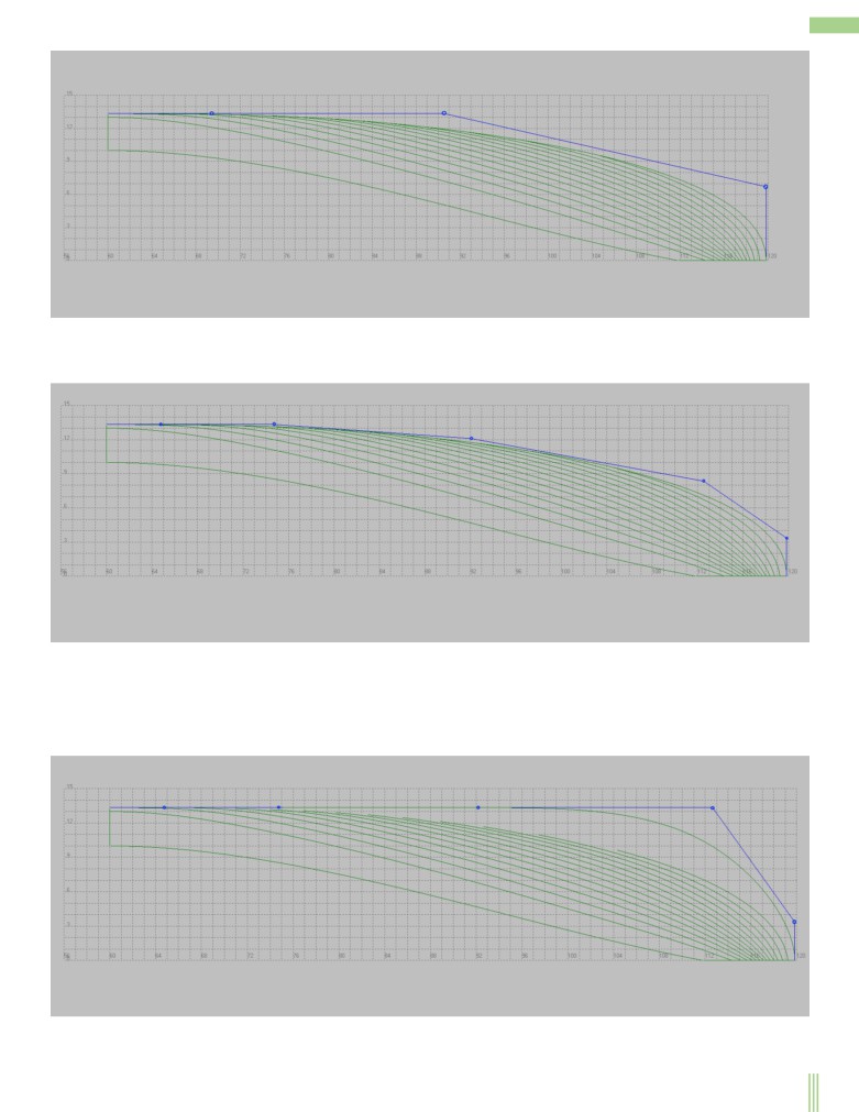
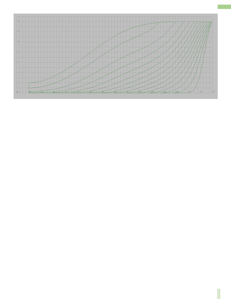
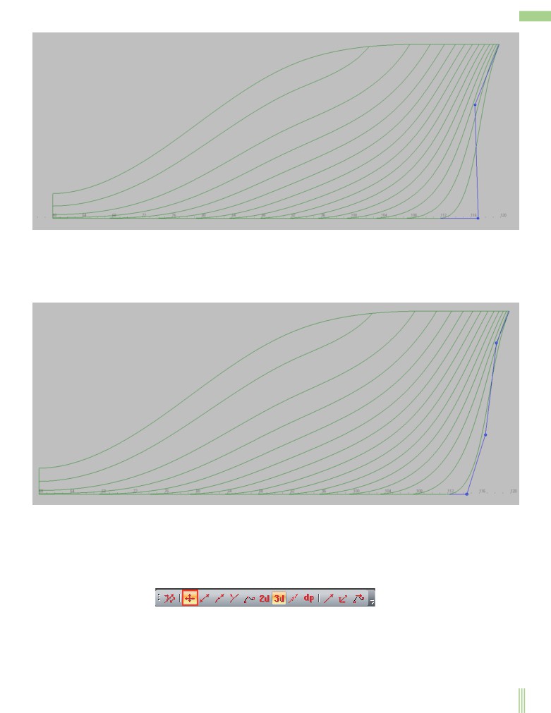
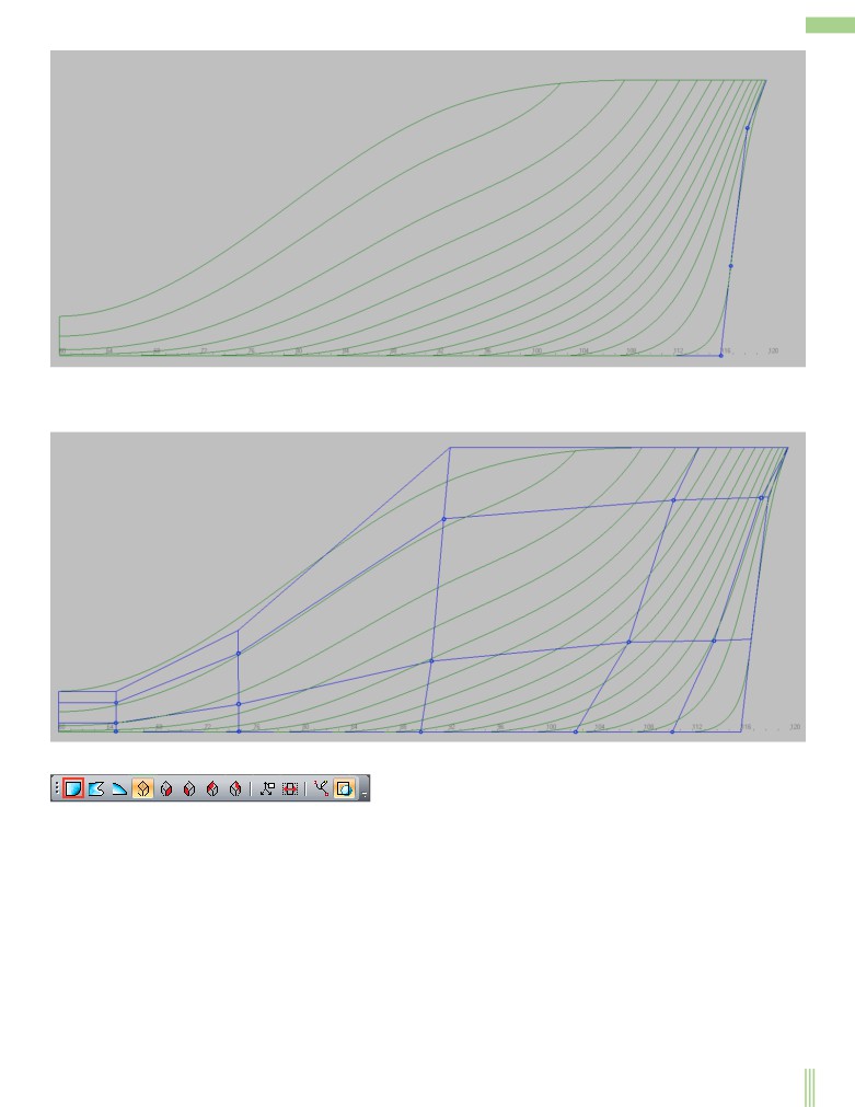
Surface intersection lines with a set of orthogonal planes.
These are curves that are obtained as a result of the intersection of a surface with a set of orthogonal planes. Depending on the current
cut plane, such planes can be frames, waterline, or buttocks. The location of these planes is determined by the grid specified in the
model or by the number of sections to the depth of the working volume. When you visualize sections on a grid, the additional sections
are rendered in yellow.
79
As well as lines of equal parameter sections are automatically rebuilt when the position of the control polyhedron points of the surface
changes.
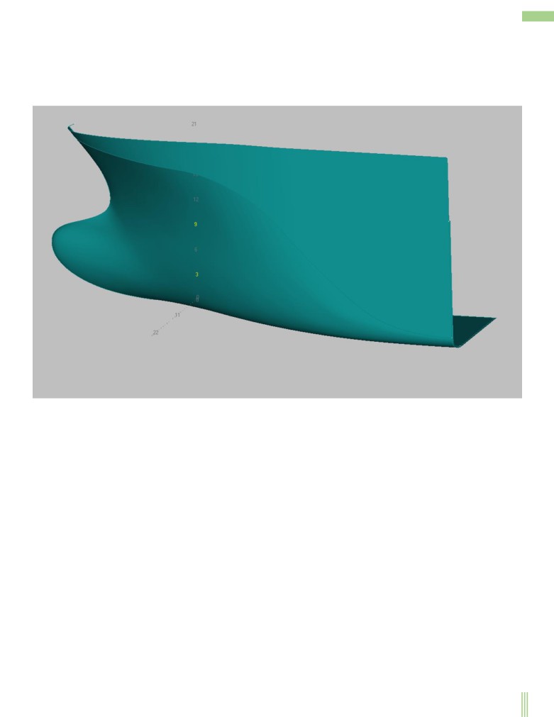
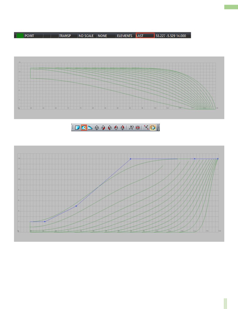
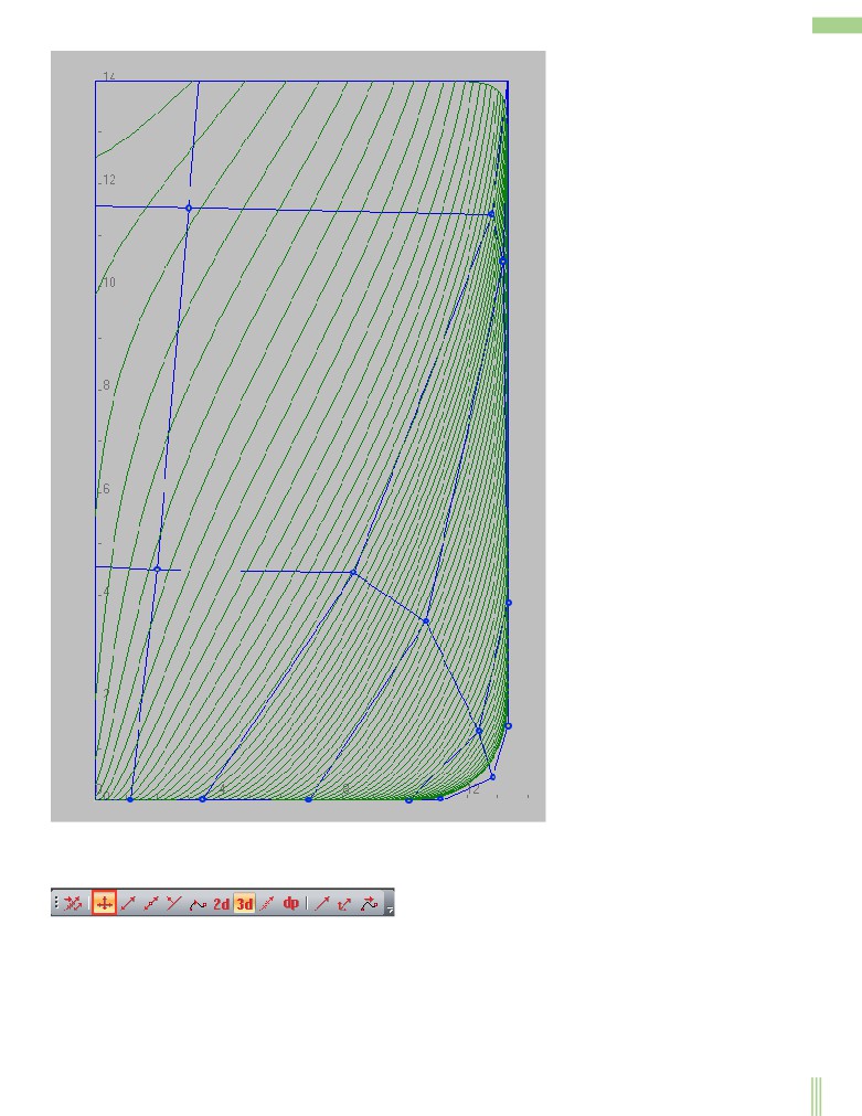
Shaded surfaces.
One of the variants of realistic representation of the hull surface. For ease of presentation, surfaces can also be represented as semi-
transparent.
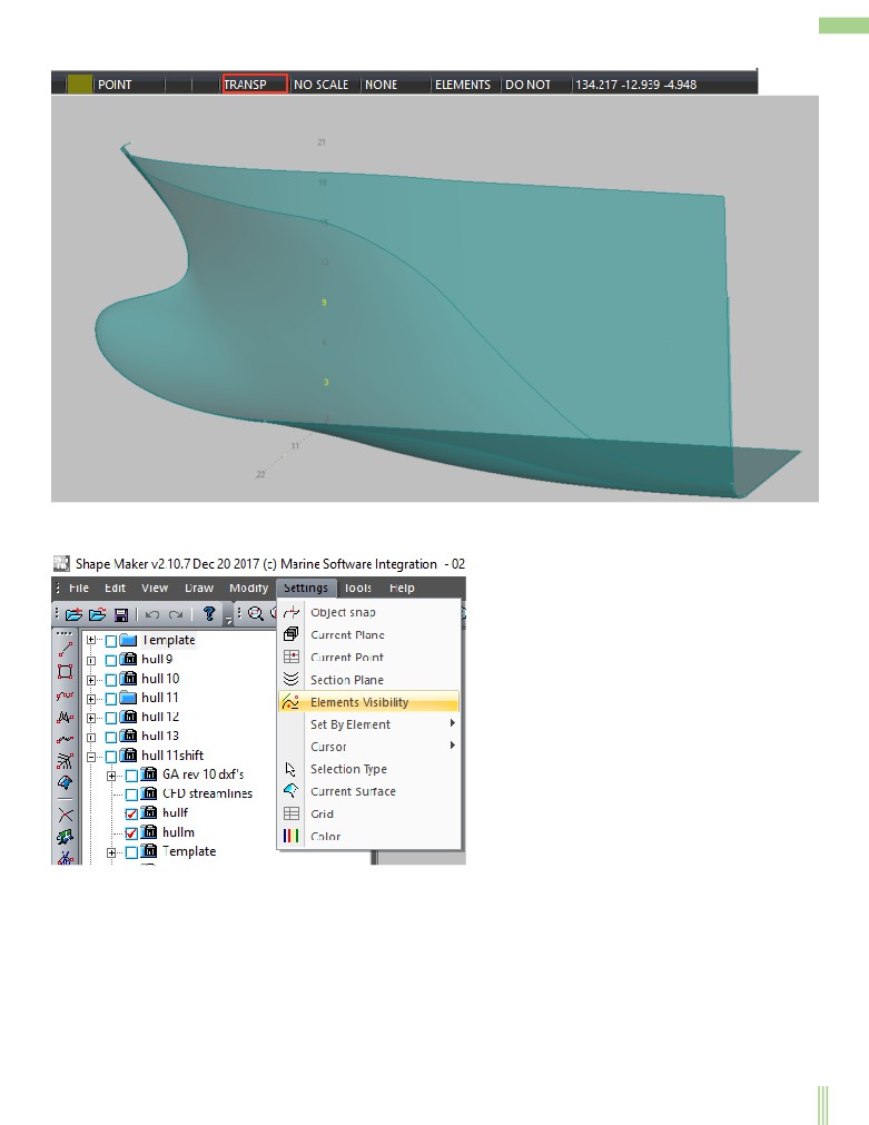
80
For this purpose it is necessary to click the mouse in the corresponding field status bar.
Note, That all three of the above visualizations are not separate objects in the system. For example, lines of equal parameter or section
are not lines, That can be edited or deleted. You can change the shape of these lines only by changing the position of the polyhedron
surface control points. All three surface options can be enabled at the same time using the following command.
81
В диалоговом окне.
can also be done by pressing the corresponding button from the toolbar Levels:
Edit surfaces.
The process of editing a surface patch shape is similar to editing a curve. The difference is, That the surface case is a 2d case. Control
polyhedron points affect a specific area of surface change and stand from the surface slightly farther than in the case of the line. When
there are quite a big number of control points on a surface area, changing the position of one control point results in a local change in
the surface shape.
To edit a surface, it is enough to click inside a contour of a surface formed boundary lines. After you select a surface to edit, the
control polyhedron points appear. Modification of the position of the control polyhedron points is the basic method of surface
smoothing. Only the internal points of the control polyhedron are available for editing. The corner points of the control polyhedron
can only be modified when the position of the corner point of the surface contour changes. The same can be said about the boundary
points of the control polyhedron. Their position depends on the shape of the boundary curve and changes only when the boundary
curve changes.
82
Changes the position of corner points on the surface.
As shown in the case of line editing, the line and surface points form a single topological system. Therefore, as with editing the end
point of a line, editing the corner point of the surface will change the shape of the boundary lines and surface. Changing the shape of
the surface in this case depends on the mode of the form change. So, the picture below shows how to change the form in:
In this case, only the position of the line endpoint and the corner point of the surface changes.
83
If you select the following form edit mode:
The position of all control points adjacent to this point of the lines and all the control points of the surface, except the bounding
boundaries, will be recalculated by linear rule.
84
In the case of the next editing mode:
The tangents will be saved in the end Boundary curves and tangents on the surface boundary to be changed. All intermediate points of
curves and surfaces will be recalculated by linear law.
This mode is useful if you want to change the position of the corner point, but still keep tangents of the surfaces that are coming to that
point.
85
Also, as with the modification of the line for the surface, you can set the modification mode of the surface part.
The following settings will result in a partial surface modification.
As you can see from this example, only a subset of the surface control points are changed.
Changes the shape of a surface boundary line.
Changing the shape of a boundary curve affects the position of the control polyhedron points in the same way that a corner point
changes. So with the same editing mode settings as in the previous case, the result will be the same.
It is important to note that if you change the shape of the boundary curve, all surfaces that are based on this curve will be modified
according to the selected edit mode. At the same time there are no gaps and cracks on the border of two surfaces.
86
Changes the position of the control polyhedron points on the surface.
In order to start editing the surface just click the mouse inside the contour formed by the boundary lines of the surface. Changing the
position of the control polyhedron points will change the shape of the surface.
The control polyhedron of a surface is similar to a control polygon of a line and has similar properties. Consider some of them:
- The locality of the surface change. In the case of a sufficiently large number of control polyhedron points, changing the position of
one of them will result in a local change of the surface shape.
- Tangent to the boundary of the surface. The shape of the surface near the border, tangents, and inclination angles are determined by
the closest to the boundary points of the control polyhedron.
- Plane. If all control polyhedron points belong to the same plane, the surface is a plane.
- Cylindrical and cone surfaces. And if all the rows of control points in one direction is on a straight line, the surface will be a
cylinder or a cone depending on the shape of the opposing border.
- Properties of the bulge of the control polyhedron. Convex control polyhedron Specifies a convex area of the surface without dents
and inflections.
As well as for the points of the control polygon of the line, For the surface there are several different ways to modify the control
polyhedron. The simplest is to change the position of one checkpoint. The editing mode must be set as follows:
The following shows how to edit a single control point.
If the surface has a sufficiently large number of control points and is already smoothed, you can edit the group of control points. The
changes will not only affect the points selected for editing, but also the point group around the point. The position of these points is
calculated from the condition of maintaining the maximum smoothness of the surface. To edit a point group, select the following
mode:
As with editing a point group on a line, the option S:1 Indicates how many rows of points around the selected point will change during
the editing process. So, in our example, this is one row of points. For the user's convenience, the lines connecting the editable points
are highlighted in a different color.
87
It is also important to note another feature of this method of surface editing. Often, when you edit a point group, you can incorrectly
change the coordinates of the points adjacent to the surface boundary and define the smooth connection with the other surface. If you
edit a surface group with the following mode enabled, the points adjacent to the surface boundary will not be edited.
Changing the shape of a surface when the position of the control polygon points changes dynamically appears on the screen. As
mentioned earlier, a surface shape can be represented as lines equal to a parameter, orthogonal sections, and shaded surfaces. Each of
these views changes dynamically. In addition to this, the editable surface can be visualized by the curvature graphs of orthogonal
sections and inflection lines by frames, waterlines, and buttocks. Curves and inflection lines also change dynamically when the
position of control points changes. This allows you to quickly control the shape of the surface.
88
You can show a graph of curvature radii and inflection lines using the following command:
or from the toolbar Modify:
89
In the menu Options You need to include the following options:
If these options are enabled, the inflection lines and curvature curves will be shown for each currently editable surface.
90
Below is an example of the inflection lines visualization and the section curvature graph.
The program provides a fairly wide set of commands for operations with points of the control polyhedron surface. Surface smoothing,
control point area editing, or flatended rows of surface control points are described in the user's Guide. In this tutorial, we will
consider these commands as needed.
Smooth connection of surface patches.
Sometimes, in the process of modeling the surface smoot surface patches connection is reqired. The following example shows that the
patch of the surface of the aft ship of the hull should be smooth smoot with the surface of the fore ship along the line of the
midsection. Before joining surfaces, it is necessary to make smooth connection of longitudinal lines among themselves. In our case it
is a line of a flat side and a inclided flat bottom. The commands of smooth joining of lines were described in section “Working with
lines”. Another prerequisite for a smooth connection of two surfaces is the existence of a common boundary line.
91
For smooth joining of surface patches on common boundary line use the following commands
or from the toolbar Modify:
In the dialog box that appears, select the following option.
Then you specify the common boundary of the surface and the connected surface. After that the closect to the common boundary
control points will be exposed in such a way as to ensure smooth connection of these surfaces.
92
Straightening a number of surface control points.
One of the most common tasks in modeling flat or bar surfaces is to flatness the rows of control points in one direction. The example
below shows the location of the surface control points to flatness.
93
Use the following command to flatness the control point rows.
or from the toolbar Modify
Select the appropriate options in the dialog box that appears.
After that it is necessary to click on the lines connecting two control points in order to show the direction of the flatness.
94
The following shows the location of the control points after flatness in the longitudinal direction.
As mentioned earlier, the condition for building ruled surface are straight forming lines in the same direction. The straightening of the
control point rows is what makes this possible.
If you want to quickly reroute a row or a part of control points only on the current projection, you can click the mouse with the key
Ctrl to one of the points, then click on the second point. After that, row of points between the selected points will be straight on this
projection.
Smooth connection of surfaces with orthogonal planes.
In the practice of modeling ship surfaces, it is often necessary to smooth the curved surfaces, for example, the nasal tip with the
surface of the flat board and the flat bottom. For this purpose, it is possible to use the method of docking of two surfaces which has
been described earlier.
95
The example below shows the area of the flat side on the front projection. The image is compressed 10 times on the vertical direction.
In order to smoothly connect the surface of the fore ship with a flat side, it is necessary to expose the vertical tangent to the line of the
flat side. The easiest way is to click with the mouse and press Ctrl On each line between the boundary point and the closest surface
control point. This will change the position of the control point so that the tangent in that area of the surface will be vertical.
96
The result after editing the surface control points in the area of the flat side. The image is compressed 10 times on the vertical axis.
Surface smoothing.
Surface smoothing is the most laborious process, consisting in distribution of points of control polyhedron of a surface so that to
satisfy conditions of approach to the starting points or lines and, at the same time, to save the required smoothness and
manufacturability. For the most part, the smoothing process is manually moving the control points. The program also provides several
different commands that automate this work, where possible.
97
Most of these commands are focused when you call the next command.
or from the toolbar Modify
98
As you can see from the dialog box that appears when you click this command, there is a fairly large set of surface smoothing features.
The system allows you to smooth out both the control Point area and the row or rows of control points. In some cases, you can save
one of the projections without changing them. All of these methods will be discussed in more detail later.
As long let’s use methods are available on hot buttons.
If you click on one of the control points of the surface with the Ctrl and then select the control point change area, the system
recalculates the position of the control points within the selected area as interpolation from the boundaries of the selected area.
If you click on one of the control points of the surface with the Shift And then select the area of control points change, the system will
try to find such a position of control points, at which on the selected area of a surface the energy of deformation will be minimal. It
should be noted that this method of smoothing does not apply to the control points closest to the surface boundaries. This method
works better if you select a large number of control points.
Visualization of the curvature Chart of cross-sections and inflection lines.
Control of the surface shape during its editing is very important. To do this, the system provides visualization of curves of the
curvature of cross-sections and the line of inflection of the surface by an orthogonal section. This information provides a clear picture
of the quality of the surface. As well as sections, curvature graphs and inflection lines change dynamically when the position of the
surface control points changes. This gives you a clear picture of the correct direction of the surface control point movement.
Enabling this mode can also be done by the following command.
99
or from the toolbar Modify:
100
and selecting the appropriate mode in the dialog box.
Let's look at how this works on the side projection example.
101
The line of inflection of a surface on buttocks is a line of red color. On the projection side represented above any buttocks intersects
with the inflection line only once. This suggests that none of the buttocks on this surface will have more than one point of inflection.
The following is a case where buttocks has multiple inflection points in a very small area of the surface. This means that the surface
in the area has a defect.
102
You can remove this surface defect by changing the position of the control points in this area as shown below.
Note that on any of the projections are shown all lines of inflection by frames, waterlines and buttocks. This allows you to control the
shape of the sections across all three projections. It should be noted that, in general, the lines of inflection are not smooth. This is
because the system uses the B-spline surface of the third degree, for which, the condition of smoothness of only the first and second
derivative (the angle of inclination and curvature at each point of the surface) is fulfilled. An inflection line is a representation of a
third derivative, for which the smoothness condition is not met. But as experience shows, the smoother lines of inflection - the higher
the smoothness of the surface.
A significant change in the shape of the inflection line can be achieved even with a slight change in the position of the control points.
Therefore, it is recommended to use a scaled cursor movement when modifying the position of the control points. Often, moving the
control point to a few millimeters is enough to change the shape of the inflection line. The inflection line is a simple and reliable
means of surface quality control. The correct placement of the inflection lines on the surface guarantees no undulation on any section
of the surface. More detailed work with lines of inflections will be considered later.
103
Below is an example of visualization of frames curvature and inflection line by frames, waterlines and buttocks.
104
First project.
-The program allows to simulate the ship surface from scratch as well as from the prototype. There is no significant difference in the
approaches in either case. As the first surface modeling project, start drawing from scratch. Let's try to make a model of a monoscrew
vessel with a stern skeg and without bulbows bow, as it is shown below.
Create a new project.
As with any other program, you need to do a few preliminary steps to start a new project. All project information is contained in the
file with the extension - Shm. You can create a new project file by using the following command.
or from the toolbar Main:
105
In the dialog box, you must enter a file name and create a new Project.
The project file will then be created in the selected directory and downloaded by the program. All parameters of the new project are
set by default and the program's working window looks as shown below.
In principle, everything is ready to start working with the project, but for the convenience of work it is better to set some parameters
according to the parameters of the projected vessel.
106
Создание структуры блоков проекта.
As shown below, the new project has only one block. The same block is the current.
As mentioned earlier, all new project items will be in this current block. The block name and the structure of the project blocks can be
easily changed at any stage of design, but to properly organize the project from the beginning, We'll do it now. In order to change the
name of the block just click the left mouse button in the Block Name field and specify a new name.
Как это показано ниже.
107
Let Hull 0 will be the root block of our project. Let's create the fore ship, aft ship and parallel midbody blocks. To do this, right-click
on the block name and select the appropriate command from the drop-down menu
After that, a block with the default name will appear in our block.
Change the name as shown above. The rest of the blocks are also created in the same way.
Note that each new preset block automatically becomes current. All newly entered elements will fall into the current block.
108
In order to change the current block Just left-click on the folder icon next to the block name. Since in our example we will work first
with the fore ship will make the appropriate block current.
Specifies the grid.
Once we have decided on the structure of the project blocks, it is necessary to take one more step before the start of the work - to set
the grid of the lines drawing. The grid plays a fairly important role in the project. The maximum dimensions of the projected surface
of the vessel's hull are determined on the grid. The grid is also used to construct the hull sections of the vessel. Grid section numbers
can be used to specify point coordinates. The specified grid can also be used to output a lines drawing.
You can change the default grid value by using the following command.
or from the toolbar Settings:
109
Change the default grid value in the dialog box.
The default value grid is an option that is unlikely to be used for our purposes. So in the longitudinal direction is set 11 frames. Zero
rib is at the beginning of the coordinate system, and the last at a distance of 100 m from the beginning of coordinate systems. Spacing
between frames set to 10 m.
We introduce the following values for our project:
- In longitudinal direction -3, 72, 0.6,
- In the transverse direction 0, 9, 0.6,
- In vertical direction 0, 15, 1.
All specified values are entered in meters. The first parameter shows the position of the start section, the second parameter shows the
position of the end section, the third parameter defines spacing. The interval between the start and end sections should be equal to the
number of spacings. Otherwise, the program will generate the following error message.
The program supports almost any option to specify the grid. You can set any direction of the coordinate axes, The zero-section
position and the direction of the section numbering. Also, if necessary, You can add intermediate sections, such as intermediate
frames and additional sections. The program also supports several intervals with different spacing values. It is important to note that
the beginning of each new interval must coincide with the end of the previous one. Otherwise, the program will issue a message Error.
110
For more information about specifying a theoretical drawing grid, refer to the user's Guide.
In our case, the parameters of the lines grid are as follows:
-In longitudinal direction
111
-In transverse direction
112
-In vertical direction
When you finish editing, the grid will look like this:
113
Modeling the fore ship.
After you have made all the necessary installations to start working on the project, let's move on to the fore ship modeling. The fore
ship of our project consists of three surfaces. It is a surface of a flat bottom, a surface of a flat side, passing in a vertical cylindrical
surface in a nose and the basic curved surface.
114
Specifies the boundary lines of the curved surface area.
Let's start modeling by specifying the boundary lines of the curved surface. This is the bilge radius line, the flat bottom line, the stem
line and the flat side line passing into the contour of the deck. You can start entering boundary lines by using the following command.
or from the toolbar Create:
In the coordinate input line, enter the first point of the cheekbone line.
After that the rubber thread from the just specified point will appear on the screen. Let's continue entering the next point.
Now the line between the first and second points and the rubber thread passing from the second point will be visible on the screen.
This means that we can continue to enter the contour of our future surface. We introduce the following points sequentially.
115
As you can see on image below we have entered the bilge radius line, flat side lines, stem and flat bottom line.
In order, To set a surface, The contour must be closed. So enable topological snap to point
and select the point with which the input began.
The closed path will look as shown below.
116
Click Esc On the keyboard or right mouse button to stop entering curves.
In the first approximation, the boundary lines are straight.
Let's go to the projection Front
and edit the bilge radius line.
117
Just click the left mouse button on the bilge radius line, change the position of the control points that appeared. Point the tangents at
the end points of the bilge radius line vertically and horizontally, respectively. To do this, just set the tangents approximately, and then
refine by clicking the left mouse button with the Ctrl button pressed on the corresponding line of the control polygon. For easy editing
of the line we recommend to increase this area on a larger scale. This is achieved by rotating the mouse wheel.
After editing, the curve should look something like this.
To stop editing, press Esc On the keyboard or right mouse button.
118
Let's move on to the projection Plan
and change the shape of the flat bottom
line and the flat side.
Due to the fact that we work with fore ship we recommend to select the working volume of the fore ship of the window.
After editing, these lines should look like this:
119
Change the line of the flat side and stem.
It should be noted that unlike all other lines, the line of the flat side is a spatial line in our case. In this case, for example, when editing
on a projection Side, points of the control polygon should be moved strictly vertically. This will keep the shape of the curve on the
projection Plan. You can set the following cursor mode for orthogonal move of control points.
From the example above, you can see that the control points for making the line of the flat board of the required shape is clearly not
enough.
Add control points to the line for more freedom to edit the curve. To do this, click with the left mouse button with the simultaneously
pressed Ctrl on the line that connects the control points of the curve polygon.
The additional control point that appears will allow you to get closer to the desired result. It is desirable that the projection Side had a
horizontal tangent in connection to the top point of the stem. As mentioned above we do not want to change the shape of this line on
the projection Plan. Therefore, for the new control point, we will manually change only the vertical coordinate. To do this, you select
this point to edit and click ← or → and edit the vertical coordinate in the input string as shown below.
Since the top point of the stem has a height of 14 meters, we expose the same coordinate in the input string.
After that the curve will get more correct form.
120
In this way, our curves form a closed contour and, in the first approximation, have the required shape.
121
Sets and edits a surface patch.
You can set a surface on a closed path from the lines by using the following command.
or from the toolbar Surface:
Then, you must specify the lines that make up the path sequentially. A line that has no topological link to the previous line cannot be
selected. The selected lines are highlighted in red. After all the contour lines are selected, click Enter, And the program will create the
first surface of this project. The surface will be represented by lines of equal parameter.
122
If the selected contour is not closed, the program produces an error message.
Let's start editing our surface. Just click the left mouse button inside the contour of the surface. Consider the control polygon of the
surface.
First of all, one of the control points is not visible. This point goes beyond the allocated work volume and is not shown. In order to
increase the working volume, you can go to the projection Side by command
and allocate a large area for visualization by the command
123
After that the control polyhedron will look something like this:
As you can see from this example, when you specify a surface, the program calculates the initial position of the control polyhedron
points. The position of these points is defined as the interpolation of the adjacent control points on the boundary curves. In the
longitudinal direction on our surface two rows of control points, and transverse three rows, since three control points were set on the
flat side line. All other boundary lines have two control points. The algorithm for selecting the number of control points on the
surface was described earlier.
On projection Side our control points look like this:
124
The principle of curved surfaces modeling is quite simple. In the first stage we try to give the surface the required shape with an
existing set of control points. After all the editing capabilities are exhausted, the number of control points is gradually increased by
increasing the number of control points on one of the boundary curves. As the number of control points increases, the shape of the
surface remains virtually unchanged. The new control points provide additional options for modifying the surface locally. The more
control points on the surface, the more consuming the process of changing it, so it is very important to try to reach the required form
with a minimum set of control points and increase their number only if necessary.
Another important feature of this type of surface modeling is the correct and uniform location of the control polyhedron points.
Ideally, the longitudinal lines of the control polygon should repeat the imaginary lines of current around that surface. Vertical rows of
points should smoothly transform from midship to stem. Note also that the series of control points located in the planes frames
intuitively more understandable for editing. Therefore, it is recommended to try to expose the midsection-frame series of control
points strictly vertically. If you increase the number of control points, the new control points in this area will also be vertical and do
not require additional time to edit. The same applies to tangents in the vicinity of the midship frame, the line of the flat side and the
line of the flat bottom. It is enough to place tangents with a minimum set of control points and when adding new points tangents will
be saved.
Align the series of control points closest to the cylindrical insert and put tangents to the flat side and the flat bottom as shown below.
To set these rows vertically, you may need to adjust the position of the boundary curve points. Lines of equal parameter of a surface
give very weak representation about a form. In real life it is more necessary to work with sections. To do this, turn off the
visualization of the lines of equal parameter and enable visualization of the surface sections
125
The result will look something like this:
Try to correctly position the series of surface control points as early as possible. The new control points that you add to the surface
later will be ordered according to the existing Control point layout. The correct location of the control points significantly saves time
on giving our surface the required shape.
Let's check how our surface looks in the top view. To do this, select the appropriate projection.
Pay attention to the line of the flat side passing into the line of the boulevard. This line has a polygon with three control points. The
points closest to the endpoints determine the angle of the curve. Only one midpoint allows, you to change the shape of the curve and,
in our case, it is not enough. To more precisely define the shape of this curve, add more control points. To do this, finish editing the
surface by pressing the button Esc or right-click and select the appropriate curve for editing.
126
The simplest way to increase the number of control points on a line is to click with the mouse while pressing Ctrl one of the lines
connecting the control points to each other. This will increase the number of control points and the shape of the curve does not change.
We will use the appearing points to give our curve a more realistic shape. Put the middle and, following it, the nasal control point on
the maximum half breath of the vessel. For simplicity, use the coordinates of the points in the command line. Thus, the four most
stern control points of our curve will be on the maximum half breadth of the vessel. According to the properties of the curves
described earlier, part of the line will be the exact straight from the point of half breadth to the midship frame approximate to frame
95 in the top view. If you change only the half breadth of these points, the shape of the curve will not change in the side view.
127
It is important to remember that the surface that the edit curve is bound to remains unchanged until the user has completed the
boundary curve editing process. The curve’s editing is finished by pressing the button Esc or right-click. Before completing the curve
modification, make sure that the next Surface modification mode is enabled.
This mode will allow you to save the tangent to the edges of the surface the same as they were before you started editing line. The
result of the surface change is shown below.
Let's move on to the projection Side
and change the line of the flat board.
Increase the height of the control point of the line in the area frame 92 to 14 meters. This way the fore part of the curve will have a
horizontal area.
If you change the position of the control point, the curve in the top view remains the same. As in the previous case, the surface shape
will not change until the boundary curve is edited.
128
Now the fore ship has become more reminiscent of the form of a real vessel.
129
Let's go to the projection Front
and select the surface to edit.
From the configuration of the surface control points, we can hardly influence the shape of the surface, as most of the control points are
responsible for the tangent surfaces to the flat bottom and to the flat side. To be able to edit the surface you need to add more control
points. To do this, move on to the projection Side
, Let's refuse to edit the
surface and select the line of the buttock in CL for editing.
130
As mentioned above, you can control the number of surface control points by increasing the number of control points on the boundary
curve. In our case we want to increase the number of control points in the vertical direction. To increase the number of points on the
buttock in CL line just click with the left mouse button pressed Ctrl to the line connecting these control points. After that the
additional control point will appear on the line, and the line retains its former shape. This allows you to add control points to change
the desired curve fairly locally.
It is important to note that we could also change the number of control points on the bilge radius line when going into a parallel
midbody. Based on the experience of surface design, we recommend that you keep the minimum number of control points on the bilge
radius line. This will allow to control the number of points on the surfaces of the fore ship by the stem line in the fore part of the
vessel and the transom line in aft ship part. At the same time the number of control points in fore and aft parts of the ship can be
different and depend only on the complexity of the described surface.
Let's use the additional control point that appears and make the entrance radius to the main plane more smooth. It is recommended to
use orthogonal cursor movement.
Now stem will look something like this.
131
We finish editing the stem line and return to the editing of our surface. The appearance of an additional point on the curve resulted in
a number of points on the surface. This gives us more opportunities to change the shape of our surface.
The distribution of control points on the video side looks pretty plausible, so let's move on to the projection Front
, where we will change the position of control points.
132
Looking at the projection front can be concluded that the completeness of the frames near the flat bottom is insufficient and the radius
of entry frames in the flat bottom should be greater. Shifting to the board bottom control points, we will increase the radius of frames.
In order to keep the horizontal tangents at the entrance to the flat bottom we recommend orthogonal movement of the cursor.
133
After that, change the position of the other checkpoints roughly as shown below.
Let's move on to the projection Plan
To smooth the series of control points
in the longitudinal direction and more accurately determine the angles of entry lines.
134
The distribution of control points in the picture shown above is not ideal. The smooth distribution of control points along the surface
length will give us the smoothness of the surface itself. In addition to this change the control points that are responsible for the angle
of entry lines in the flat bottom plane. After editing, the location of the control points should look something like this.
On this we shall assume that we have finished with the curved surface of the fore ship in the first approximation. Advanced surface
smoothing techniques will be considered separately.
Specifies the surfaces of the flat board and the flat bottom of the fore ship.
For construction of a surface of a flat side first we shall set a connection line of a flat side to a parallel midbody.
However, it is important to use the topological snap mode to the point
. We build a vertical line from the upper point of
the bilge line to the maximum height of the board (15m). It is recommended to draw a line from the object snap at the bottom point of
line and edit the second coordinate in the coordinate input window. To do this from the toolbar Create:
Selects the line build mode. Specifies the bottom point, and the upper
coordinates are entered as shown below.
135
The line will look like the following.
Let's build a surface on this line and a line of a flat side. Use the Surface construction mode from the toolbar Surface:
And we'll specify the line of the flat side and the vertical line of the junction of the flat side to the cylindrical insert. This will highlight
the lines in red. It is important to note that if the selected lines do not have a common point, the subsequent line will not be allocated.
136
The surface will be built on two selected lines if you press the Enter.
Change the height of the upper fore point of the new surface. To do this, select the following form edit mode:
At the same time all control points adjoining to this point of lines and all control points of a surface, except for the bounding borders
will be recalculated by linear rule.
Select the point to Edit and enter the following coordinates in the coordinate input buildings.
The resulting surface is shown below.
Select to edit the top curve of the new surface and straighten it. To do this, click the left mouse button and press Ctrl To the start point
of the curve, and then click the end point, but no longer the key Ctrl.
137
The resulting surface will look like this.
To build the surface of the flat bottom, let's move on to the projection Side
Also, as in the case of the connection line of the flat side to the parallel midbody, we will build a connection line of flat bottom. In this
case, we will use the topological snap mode to the point
. Let's build a vertical line from the bottom point
of the bilge line to the CL plane. It is recommended to draw a line from the object snap at the bottom point and edit the second
coordinate in the coordinate input window. To do this from the toolbar Create:
Selects the line build mode. Specifies the top point, and the bottom
coordinates are entered as shown below.
After that, without stopping entering the line, left-click on the point of the connection line of the flat bottom
to the stem and finish entering the lines.
It remains only to specify a triangular section of a surface limited by a line of a flat bottom, a connection line of flat bottom to parallel
midbody and a line of a CL plane. Use the surface construction mode from the toolbar Surface:
And we'll specify the
flat bottom line, a connection line of flat bottom to parallel midbody, the line in CL and press Enter. This command creates the surface
of the flat bottom. Note that the sequence of boundary lines is important for the triangular areas of the surface. For refinements, we
recommend that you refer to the Surface setting section.
138
So the resulting surface of the fore ship will look in the isometric projection with the included section and shaded surface modes.
Modeling of parallel midbody surface.
Before you start modeling a parallel midbody set the appropriate block current. In order to change the current block just left-click on
the folder icon next to the block name.
Define the position of the aft limit of parallel midbody as 28.8 meters from the stern perpendicular and make a line of parallel
midbody in CL. Let's move on to the projection Plan
and in topological snap
to point mode
Let's build a horizontal line from
the point of the flat bottom line in the CL.
139
Once again, use the toolbar Create:
и Choose Mode Build Line. First
indicates the point Flat bottom lines in the head plane, and the coordinates of the next point are entered as shown below.
As a result, the line should look like this:
Let's go to one of the isometric projections
and use the extrusion driver to
build a cylindrical surface.
140
You can call the driver Extrusion command from the menu
or from the toolbar Drivers:
Select the type of Extrision driver from the menu that appears and press Ok.
Then specify the line that defines the direction of extrusion:
In our case it will be the newly entered line.
And then specify the forming lines
and press Enter as shown below.
141
The result of this command will be the surface of the cylindrical part of our vessel.
142
Simulation of aft ship.
Also, as in the case of modeling a parallel midbody, you must change the current block first.
Modeling of the main surface of the aft ship.
The modeling of the stern part is to begin with the construction of a flat side line. To do this, move on to the projection Side
. If the frames grid is not visible, we recommend setting the window by the
grid
Define the position of the stern point of the line of the flat board as -3, 8, 7.98 (All dimensions in meters) as well as in previous cases
of line construction, let's move to topological snap to point
Build a line from the top of the bilge line of the
cylindrical part to the transom line. Once again, use the toolbar Create:
and select the line construction mode. First indicates the point the top point of the bilge line, and the coordinates of the next point are
entered as shown below.
The result will look like this:
Put the horizontal tangent at the point of connection to cylindrical part. To do this, select the line to be edited and click with the left
mouse button Ctrl To the line connecting the end point of the curve to the nearest control point.
143
Also, as in the case of a parallel midbody to build a aft ship surface, use the Extruding driver. Call the appropriate command from the
toolbar Drivers:
Select in the pop-up driver type menu and press Ok.
Then we'll specify the line that defines the direction of extrusion:
In our case it will be a flat board line.
And then specify the forming lines - the bilge line and the flat bottom line.
and click Enter.
144
After that, we finish the surface of the flat side by analogy with the surface of the flat side in the fore.
Use the Surface construction mode from the toolbar Surface:
and we'll specify the line of the flat board and the
vertical line of the junction of the flat side to the cylindrical part. This will highlight the lines in red.
After pressing Enter The next surface should appear.
Edit the upper edge of the surface of the flat board similar to the fore ship. Change the coordinates of the top point of transom.
And straighten the top edge on the projection side.
145
It is important to remember that these adjustments are best done in
This mode gives a better distribution of the control points of the modified lines and surfaces.
In 3D our surface will look like that:
Modeling of transom.
Let's build a line from the top point of the transom to the CL. As in all previous cases, we will use the topological snap to the point
and build a horizontal line from the top point
of the transom to the CL. In the toolbar Create:
Select the line build mode.
First top point transom, and the coordinates of the next point are entered as shown below.
146
As a result, the line should look like this:
Then, without stopping entering the line, select the bottom point of the transom in the flat plane.
Now you can build a surface of transom. Use the surface construction mode From the toolbar Surface:
and specify
the horizontal line in series transom, The flat side line and the bilge line. This will highlight the lines in red.
148
After pressing the Enter The missing boundary line will be completed and a part of the transom surface is built.
We will set the missing part as a triangular section of the surface without leaving the surface setting mode.
149
On this surface transom can be considered finished.
Modelling of the surface of fodder skeg.
Let's build the surface of the stern skeg similar to the picture below.
150
Before starting a build, we recommend that you create a separate block in the block tree for skeg. To do this, click Right-click on the
Block “Aftship” In the block tree window and select the following command:
Then we enter the name of the new block as shown below.
By default, the new entered block will be current, and all newly-set elements will be in this block.
151
Let's start the construction with the flat bottom line of skeg. Let's take the half breadth bottom skeg 1.5 m. and build a horizontal line.
To do this from the toolbar Create:
Selects the line build mode. Specifies
the top point, and the bottom coordinates are entered as shown below.
The fore point of our line will be based on the underside line of the stern border of the cylindrical part of the vessel.
Therefore, select the following mode to move the cursor orthogonally:
Another important feature of the construction of this line is that the fore point should be topologically associated with the line of
cylindrical part. To do this, use the topological link mode to the line.
And, after that Click left button of a mouse on a
stern underside a line of a cylindrical part. Because the orthogonal move of the cursor is enabled at the same time as the line reference,
the new point connected to the line will have a fixed coordinate snap Y. That is if you change the shape of the line that hung the point,
the coordinates of the point will be counted so that Y coordinate remained unchanged. As a result, the new line will look like the
following.
Let's build the curved part of the skeg. Select the topological snap to point mode
and begin a new line from the stern point line of the flat part of the skeg. The second point of the new line set as it is shown below.
¨
Before you build this line, do not fordget to turn off orthogonal cursor mode. The easiest way to do this is to press the F9.
After that, do not stop entering the make line at the point of the stern bilge line of the cylindrical part in CL.
Let's go to one of the isometric projections
and use the pull driver to build
the side surface of the skeg.
152
Select the desired option
And start the driver. As a guide line select
the line skeg in CL.
Then we set up the driver lines. As forming use the lines of flat bottom skeg.
153
The resulting surface of the driver is shown below.
154
Let's build a surface of a flat bottom skeg. Use the Surface construction mode from the toolbar Surface:
and set the
contour lines of the surface.
155
Then press Enter:
As it was seen from the constructions the surface of the skeg intersects with the surface of the main body. Let's build the intersection
lines and cut down on these lines of the surface of the skeg and the hull. To make the intersection lines differ from the other lines
select the appropriate color. The easiest way to change the current color is to click in the corresponding field status bar,
and select a new current color in the dialog box that appears.
Next, select the mode to draw the intersection line from the toolbar Create:
156
and specify the surfaces to intersect. In our case it is the surface of the
body and the surface of the skeg driver. The intersection line will look like this:
Then select the surface trimming mode from the toolbar Cut:
and cut the skeg surface by sequentially specifying the trim
path.
161
Then cut off the surface of the main body.
163
Similarly, trim surfaces by cutting the line by selecting the appropriate mode from the toolbar Cut:
And specifying the
area of the line must be trimmed from point to point. After trimming the lines of the hull will look like: